4 Numerical Methods

4.1 Introduction

In this section we will be discussing on numerical methods for solving algebraic and transcendental equations. An expression of the form $f(𝑥)$ = ${a_0}$𝑥^𝑛+${a_1}$𝑥^𝑛−1 + ⋯ + ${a_n−1}$𝑥 + ${a_n}$,$a_0 ≠ 0$ is called a polynomial of degree ’𝑛’and the polynomial $𝑓(𝑥) =0$ is called an algebraic equation of 𝑛^𝑡ℎ degree. If $𝑓(𝑥)$ contains trigonometric, logarithmic or exponential functions, then $𝑓(𝑥) = 0$ is called a transcendental equation. For example x²+2sin𝑥+𝑒^𝑥 = 0 is a transcendental equation. If $𝑓(𝑥)$is an algebraic polynomial of degree less than or equal to 4, direct methods for finding the roots of such equation are available. But if $𝑓(𝑥)$ is of higher degree or it involves transcendental functions, direct methods do not exist and we need to apply numerical methods to find the roots of the equation $𝑓(𝑥) = 0$.

4.1.1 Some useful results

If 𝛼 is root of the equation $𝑓(𝑥) = 0$, then $𝑓(𝛼 ) = 0$
A root of an equation $f(x)=0$ is the value of x, say $x=α$
Every equation of 𝑛^𝑡ℎ degree has exactly 𝑛 roots (real or imaginary)
Intermediate Value Theorem: If $𝑓(𝑥)$ is a continuous function in a closed interval $\left\lbrack a,b \right\rbrack$ and $\left.𝑓(𝑎) \&\right.𝑓(𝑏)$ are having opposite signs, then the equation $f(𝑥) = 0$ has atleast one real root or odd number of roots between $a$ and $b$.

If $𝑓(𝑥)$ is a continuous function in the closed interval $\left\lbrack a,b \right\rbrack$ and $\left.𝑓(𝑎)\&\right.𝑓(𝑏)$ are of same signs, then the equation $𝑓(𝑥) = 0$ has no root or even number of roots between 𝑎and 𝑏.
A number α is a simple root of $f(x) =0$, if $f(α)=0$ and $f'(α) ≠ 0$, then we can write $f(x)$ as, \[f(x)=(x-α)g(x), g(α)≠0\]
A number α is a multiple root of multiplicity m of $f(x) =0$, if $f(α)$=$f'(α)$=$\cdots$=$f^{m-1}(α)= 0$ and $f^{m}(α)$= 0, then $f(x)$ can be written as, \[f(x)=(x-α)^{m}g(x), g(α)≠0\]
A polynomial equation of degree n will have exactly n roots, real orcomplex, simple or multiple.
A transcendental equation may have one root or infinite no. of roots depending on the form of $f(x)$.

4.2 Methods for finding the root

The methods for finding the roots of $f(x)=0$ are classified as

Direct methods
Numerical methods

Direct methods give the exact values of all the roots in a finite number of steps.

Numerical methods are based on the idea of successive approximations. In these methods we start with one or two initial approximations to the root and obtain a sequence of approximations $x_1,$$x_2,$,$x_3,$,$\cdots$$,x_k$ which in the limit as $k\to\infty$ to the exact root $x=a$.

There are no direct methods for solving higher degree algebraic equations or transcendental equations. Such equations can be solved by Numerical methods.

In theses methods, we first find an interval in which the root lies. If a and b are two numbers such that f(a) and f(b) have opposite signs, then a root of $f(x)=0$ lies in between a and b. We take a or b or any value in between a or b as first approximation $x_1$. This is further improved by numerical methods.

Order of convergence: For any iterative numerical method, each successive iteration gives an approximation that moves progressively closer to actual solution. This is known as convergence. Any numerical method is said have order of convergence $𝜌$, if $𝜌$ is the largest positive number such that $|𝜖_{𝑛+1}|≤{𝑘}{|𝜖_{𝑛}|}^𝜌$ , where $𝜖_𝑛$ and $𝜖_{𝑛+1}$ are errors in $𝑛^{𝑡ℎ}$ and $(𝑛 + 1)^{𝑡ℎ}$ iterations, $𝑘$ is a finite positive constant.

4.3 Numerical Methods for finding root

4.3.1 Bisection Method (or Bolzano Method)

Bisection method is used to find an approximate root in an interval by repeatedly bisecting into sub intervals. It is a very simple and robust method but it is also relatively slow. This methods is based on the intermediate value theorem for continuous functions.

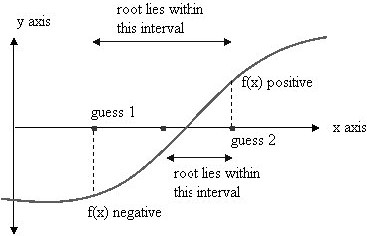
Figure 4.1: Figure showing Bisection method

4.3.1.1 Algorithm:

Let $𝑓(𝑥)$ be a continuous function in the interval $\left\lbrack a,b \right\rbrack$ and $\left.𝑓(𝑎)\&\right.𝑓(𝑏)$, such that $𝑓(𝑎)$ and $𝑓(𝑏)$ are of opposite signs, i.e. ${𝑓(𝑎)𝑓(𝑏)} < 0$, then there will be a root of $f(x) = 0$ in between a and b.

Step 1 : Let the first approximation be the mid point of the interval $(a,b)$. i.e.,

\[x_{1} = \frac{a + b}{2}\]

If $f(x_1)= 0$, then $x_1$ is a root.
Otherwise root lies between $a$ and $x_1$ or $x_1$ and $b$ according as $f(x_1)$ is positive or negative.
Then again we bisect the interval and continue the process until the root is found to desired accuracy.
Let $f(x_1)$ is positive, then root lies in between $a$ and $x_1$, then the second approximation is given by,

\[x_{2} = \frac{a + \ x_{1}}{2}\]

Let $f(x_2)$ is positive, then root lies in between $a$ and $x_1$, then the second approximation is given by,

\[x_{3} = \frac{x_{2} + \ x_{1}}{2}\]

Similarly, we get other approximations.

Remarks:

Convergence is not unidirectional as none of the end points is fixed. As a result convergence of Bisection method is very slow.
Repeating the procedure 𝑛 times, the new interval will be exactly half the length of the previous one, until the root is found of desired accuracy (error less than ∈). Therefore and at the end of$𝑛^{𝑡ℎ}$ iteration, the interval containing the root will be of length $\frac{|b-a|}{2^n}$, such that $\frac{|b-a|}{2^n}|<∈$ ⇒ $\log\frac{|b-a|}{2^n}|<∈$ ⇒ $\log{|𝑏 − 𝑎|}− log {2^𝑛}< log ∈$ ⇒ $\log{|𝑏 − 𝑎|}− log ∈ < n log 2$ ⇒ $𝑛 > \frac{log |𝑏−𝑎|−log ∈}{log2}$

∴ In bisection method, the minimum number of iterations required to achieve the desired accuracy (error less than ∈) are

\[n\ \geq \ \frac{\log\frac{|b - a|}{\in}}{\log{\ 2}}\]

4.3.1.2 Examples

Example 1

Find a real root of the equation $f(x) = x^{3}-x-1=0$ using Bisection method?

Solution

First find the interval in which the root lies, by trail and error method

\[f(x) = x^{3}-x-1\]

\[f(0) = -1\]

\[f(1) = -1\]

\[f(2) = 5\]

Here, $f(1) = -1$ and $f(2) = 5$

i.e, $f(1) . f(2) = -5 <0$

∴ A root of $f(x)=x^{3}-x-1 =0$ lies in between 1 and 2.

First approximation

$a = 1,b=2$ $x_{1} = \frac{a + b}{2}$ =$\frac{1 + 2}{2}$ = 1.5

$f(x_1)$ = $f(1.5)$ = $(1.5)^{3}-1.5-1$ = $0.875$, which is positive

Hence the root lies in between 1 and 1.5

Second approximation

$a = 1, b=1.5$

$x_{2} = \frac{a + x_{1}}{2}$ = $\frac{1 + 1.5}{2}$ = $1.25$

$f(x_2)$= $f(1.25)$ = $(1.25)^{3}-1.25-1$ = $-0.29$, which is negative

Hence the root lies in between 1.25 and 1.5

Third approximation

$a = 1.25, b=1.5$

$x_{3} = \frac{x_{2} + b}{2}$ = $\frac{1.25 + 1.5}{2}$ = 1.375

$f(x_3)$ = $f(1.375)$ = $(1.375)^{3}-1.375-1$ = $0.224$, which is positive

Hence the root lies in between 1.25 and 1.375

Similarly we get $x_4=1.3125, x_5=1.34375, x_6=1.328125$ etc.

Example 2

Find a Find a root of $f(x)=xe^{x}-1=0$, using Bisection method, correct to three decimal places.

SOLUTION

$f(0) = 0.e^0-1=-1$< 0 (negative)

$f(1) = 1.e^1-1 = 1.7183 > 0$(positive)

Hence a root of $f(x) = 0$ lies in between 0 and 1.

\[x_{1} = \frac{0 + 1}{2} = 0.5\]

$f(0.5) = 0.5 e^{0.5}{-1} = -0.1756$

Hence the root lies in between 0.5 and 1

\[x_{2} = \frac{0.5 + 1}{2} = 0.75\]

Proceeding like this, we get the sequence of approximations as follows

$x_3= 0.625$

$x_4= 0.5625$

$x_5= 0.59375$

$x_6= 0.5781$

$x_7= 0.5703$

$x_8= 0.5664$

$x_9= 0.5684$

$x_{10}= 0.5674$

$x_{11}= 0.5669$

$x_{12}= 0.5672$

$x_{13}= 0.5671$

Hence, the required root correct to three decimal places is, $x=0.567$.

Example 3

Using bisection method find an approximate root of the equation $\sin x = \frac{1}{x}\ $ correct to two decimal places.

Solution: \[𝑓(𝑥) = 𝑥sin 𝑥 − 1\]

Here $f(1) = sin (1) − 1 = −0.1585$ and $𝑓(2) = 2sin 2 − 1 = 0.8186$

Also 𝑓(𝑥)is continuous in $\left\lbrack 1,2 \right\rbrack$ ∴ Atleast one root exists in $\left\lbrack 1,2 \right\rbrack$

Initial approximation:

$a = 1, 𝑏 = 2$

$x_{0} = \frac{1 + 2}{2} =1.5$ $𝑓(1.5) = 0.4963$, $𝑓(1). 𝑓(1.5)< 0$

First approximation:

$ = 1, 𝑏 = 1.5$

$x_{1} = \frac{1 + 1.5}{2}=1.25$ $𝑓(1.25) = 0.1862$, $𝑓(1).𝑓(1.25)< 0$

Second approximation:

$𝑎 = 1, 𝑏 = 1.25$

$𝑥_{2}=\frac{1+1.25}{2}= 1.125$, $𝑓(1.125) = 0.0151$, $𝑓(1). 𝑓(1.125)< 0$

Third approximation:

$𝑎 = 1, 𝑏 = 1.125$

$𝑥_{3}=\frac{1+1.125}{2} = 1.0625$, $𝑓(1.0625) = −0.0718$, $𝑓(1.0625).𝑓(1.125)< 0$

Fourth approximation:

$𝑎 = 1.0625, 𝑏 = 1.125$

$𝑥_{4}=\frac{1.0625+1.125}{2}= 1.09375$, $𝑓(1.09375) = −0.0284$, $𝑓(1.09375).𝑓(1.125)<0$

Fifth approximation:

$𝑎 = 1.09375, 𝑏 = 1.125$

$𝑥_{5}= \frac{1.09375+1.125}{2} = 1.10937$, $𝑓(1.10937) = −0.0066$, $𝑓(1.10937). 𝑓(1.125)<0$

Sixth approximation:

$𝑎 = 1.10937, 𝑏 = 1.125$

$𝑥_{6}=\frac{1.10937+1.125}{2}= 1.11719$, $𝑓(1.11719) = .0042$, $𝑓(1.10937). 𝑓(1.11719)<0$

Seventh approximation:

$𝑎 = 1.10937, 𝑏 = 1.11719$

$𝑥_{7}=\frac{1.10937+1.11719}{2}= 1.11328$, $𝑓(1.11328) = −.00120$

Hence 1.11328 is the real root correct to two decimal places.

4.3.2 Regular False Method

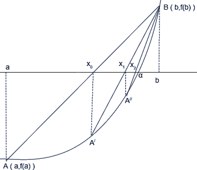
Figure 4.2: Figure showing Regular False method

Regula-Falsi method is also known as method of false position as false position of curve is taken as initial approximation. Let $y=f(x)$ be represented by the curve AB. The real root of equation $f(x) = 0$ is α as shown in figure. The false position of curve AB is taken as chord AB and initial approximation x_1 is the point of intersection of chord AB with x-axis. Successive approximations x2, x3, ………….. are given by point of intersection of chord A’B, A”B,……. with x-axis, until the root is found to be of desired accuracy.

Now equation of chord AB in two-point form is given by: \[{𝑦 − 𝑓(𝑎)}= \frac{𝑓(𝑏)−𝑓(𝑎)}{b-a}{(𝑥 − 𝑎)}\]

To find $𝑥_1$ (point of intersection of chord AB with 𝑥 - axis), put 𝑦=0

⇒ \[−𝑓(𝑎) = \frac{𝑓(𝑏)−𝑓(𝑎)}{b-a}{(𝑥_{1}− 𝑎)}\] ⇒ \[\frac{-f(a)(b-a)}{f(b)-f(a)}=(x_1-a)\] ⇒ \[(x_1−a) = \frac{−(𝑏−𝑎)𝑓(𝑎)}{f(b)-f(a)}\] ⇒ \[ x_1 = a-\frac{(b-a)f(a)}{f(b)-f(a)}\]

Repeat the procedure until the root is found to the desired accuracy.

Remarks:

Rate of convergence is much faster than that of bisection method.
Unlike bisection method, one end point will converge to the actual root 𝑎, whereas the other end point always remains fixed. As a result Regula- Falsi method has linear convergence.

4.3.2.1 Examples

Example 1

Apply Regula Falsi method to find a root of the equation $x^3+x-1=0$ correct to two decimal places.

Solution: \[𝑓(𝑥) = 𝑥^{3} + 𝑥 − 1\]

Here $𝑓(0) = −1$ and $𝑓(1) = 1$ ⇒ $𝑓(0). 𝑓(1)< 0$

Also 𝑓(𝑥)is continuous in $\left\lbrack 0,1 \right\rbrack$, ∴ atleast one root exists in $\left\lbrack 0,1 \right\rbrack$

Initial approximation

\[x_{0} = a - \ \frac{(b - a)}{f(b) - f(a)}\ f(a)\]

a = 0, b=1

${ x}_{0} = 0 - \frac{(1 - 0)}{f(1) - f(0)}\ f(0) = 0.5$

$f(0.5) = -0.375$, $f(0.5).f(1)<0$

First approximation

a = 0.5, b=1

${x}_{1} = 0.5 - \frac{(1 - 0.5)}{f(1) - f(0.5)}\ f(0.5)= 0.636$

$f(0.636) = -0.107$, $f(0.636).f(1) <0$

Second approximation

a = 0.636, b=1

${x}_{2} = 0.636 - \frac{(1 - 0.636)}{f(1) - f(0.636)}\ f(0.636)= 0.6711$

$f(0.6711) = -0.0267$, $f(0.6711).f(1)<0$

Third approximation

a = 0.6711, b=1

${ x}_{3} = 0.6711 - \frac{(1 - 0.6711)}{f(1) - f(0.6711)}\ f(0.6711)= 0.6796$

First 2 decimal places have been stabilized, hence 0.6796 is the real root correct to two decimal places

Example 2

Determine the root of the equation $\cos{x - \ e^{x}}= 0$ by the method of False position correct to two decimal places.

Solution:

$f(x) = cos x-xe^x$

$f(0) = cos 0-0e^{0}=1$ $f(1) = cos 1-1e^{1}= -2.177979523$

a = 0 and b = 1, the root lies in between 0 and 1

$x_1= 0.3146653378$

$f(x_1) = f(0.314653378) = 0.51986$

Therefore, the root lies in between 0.314653378 and 1

$x_2= 0.44673$

Similarly,

$x_3= 0.49402$

$x_4= 0.50995$

$x_5= 0.51520$

$x_6= 0.51692$

First 2 decimal places have been stabilized, hence 0.51692 is the real root correct to two decimal place

4.3.3 Newton Raphson Method

This is another important method. This method named after Isaac Newton and Joseph Raphson is a powerful technique for solving equations numerically.

Let $x_0$ be approximation for the root of $f(x)=0$. Let $x_1=x_0+h$ be the correct root so that $f(x_1)=0$. Expanding $f(x_1) = f(x_0+h)$ by Taylor series, we get,

$f(x_1) = f(x_0+h) = f(x_0) + h f'(x_0) +\frac{h^{2}}{2!}f"(x~0~)+\cdots= 0$

For small values of h, neglecting the terms with $h^2$, $h^3$,$\cdots$ we get,

\[f(x_0) + h f'(x_0) = 0\]

and $h =\frac{- f(x_{0})}{f^{'}(x_{0})}$

$x_1~= x_0+h$

$= x_0-\frac{f(x_{0})}{f'(x_{0})}$

Proceeding like this, successive approximation $x_2, x_3,\cdots,x_{n+1}$ are given by,

${x}_{n + 1} = \ x_{n}\ –\ \frac{f(x_{n})}{f^{'}(x_{n})}$ for $n=0,1,2,.....$

Remarks:

Netwon-Raphson method can be used for solving both algebraic and transcendental equations and it can alsobe used when roots are complex.
Initial approximation x₀ can be taken randomly in the interval $\left\lbrack a,b \right\rbrack$, such that $f(a).f(b)<0$
Newton-Raphson method had quadratic convergence, but in case of bad choice of $x_0$, Newton Raphson method may fail to converge.
This method is useful in case of large value of $f^{'}(x_{n})$ i.e, when graph of $f(x)$ while crossing x-axis is nearly vertical.

4.3.3.1 Examples

Example 1

Use Newton Raphson method to find a root of the equation $x^{3} - 5x + 3 = 0$ correct to three decimal places.

Solution

$f(x) = x^{3\ } - 5x + 3$

$f^{'}(x) = 3x^{2\ } - 5$

Here $f(0) = 3$ $f(1) = -1$

$f(0).f(1)<0$

Also f(x) is continuous in $\left\lbrack 0,1 \right\rbrack$.

Therefore atleast one root exists in $\left\lbrack 0,1 \right\rbrack$.

Initial approximation

Let initial approximation $(x_0)$ in the interval $\left\lbrack 0,1 \right\rbrack$ be 0.8

By Newton-Raphson method \[x_{n + 1\ } = x_{n} - \ \frac{f(x_{n})}{f^{'}(x_{n})}\]

First approximation

$x_{1}= x_{0} - \ \frac{f\left( x_{0} \right)}{f^{'}\left( x_{0} \right)}$ ,where $x_0 = 0.8$

$f\left( x_{0} \right) = f(0.8) = - 0.488$ $f'\left( x_{0} \right) = f'(0.8) = - 3.08$

$x_{1} = 0.8 - \ \frac{- 0.488}{- 3.08} = 0.6416$

Second approximation

$x_{2} = x_{1} - \frac{f(x_{1})}{f^{'}(x_{1})}$ , where $x_1= 0.6415$

$f\left( x_{1} \right) = f(0.6416) = 0.0561$ $f'\left( x_{1} \right) = f(0.6416) = - 3.7650$

$x_{2} = 0.6416 - \ \frac{0.0561}{- 3.7650}= 0.6565$

Third approximation

$x_{3} = x_{2} - \frac{f(x_{2})}{f^{'}(x_{2})}$ , where $x_2= 0.6565$

$f\left( x_{2} \right) = f(0.6565) = 0.0004$ $f'\left( x_{2} \right) = f(0.6565) = - 3.7070$

$x_{3} = 0.6565 - \ \frac{0.0004}{- 3.7070}= 0.6566$

Hence a root of the equation $x^{3} - 5x + 3 = 0\ $correct to three decimal places is 0.6566.

Example 2

Find the approximate value of $\sqrt{28}$ correct to three decimal places using Newton Raphson method

Solution

\[x = \sqrt{28}\]

\[x^{2\ } - 28 = 0\]

$f(x) = x^{2\ } - 28$

\[f^{'}(x) = 2x\]

Here $f(5) = -3$ $f(6) = 8$

$f(5).f(6)<0$

Also f(x) is continuous in $\left\lbrack 5,6 \right\rbrack$

Therefore atleast one root exists in $\left\lbrack 5,6 \right\rbrack$

Initial approximation

Let initial approximation $(x_0)$ in the interval $\left\lbrack 5,6 \right\rbrack$ be 5.5

By Newton-Raphson method,

$x_{n + 1\ } = x_{n} - \ \frac{f(x_{n})}{f^{'}(x_{n})}$

First approximation

$x_{1} = x_{0} - \ \frac{f\left( x_{0} \right)}{f^{'}\left( x_{0} \right)}$ ,where $x_0 = 5.5$

$f\left( x_{0} \right) = f(5.5) = 2.25$ $f'\left( x_{0} \right) = f'(5.5) = 11$

$x_{1} = 5.5 - \frac{2.25}{11}= 5.2955$

Second approximation

$x_{2} = x_{1} - \frac{f(x_{1})}{f^{'}(x_{1})}$ , where $x_1= 5.2955$ $f\left( x_{1} \right) = f(5.2955) = 0.0423$ $f'\left( x_{1} \right) = f(5.2955) = 10.591$

$x_{2} = 5.2955 - \ \frac{0.0423}{10.591}= 5.2915$

Third approximation

$x_{3} = x_{2} - \frac{f(x_{2})}{f^{'}(x_{2})}$ , where $x_2= 5.2915$

$f\left( x_{2} \right) = f(5.2915) = - 0.00003$ $f'\left( x_{2} \right) = f(5.2915) = 10.583$

$x_{3} = 5.2915 - \frac{- 0.00003}{10.583}= 5.2915$

Hence value of $\sqrt{28}$ correct to three decimal places is 5.2915.

4.3.4 Generalized Newton’s Method for Multiple Roots

Result: If $𝛼$ is a root of equation $𝑓(𝑥) =0$ with multiplicity 𝑚, then it is also a root of equation $𝑓′(𝑥) =0$ with multiplicity (𝑚−1) and also of the equation $𝑓′′(𝑥) =0$ with multiplicity (𝑚−1) and so on.

For example:

$(𝑥−1)^3= 0$ has ‘1’ as a root with multiplicity 3

$3(𝑥−1)^2 = 0$ has ‘1’ as the root with multiplicity 2

$6(𝑥−1) = 0$ has ‘1’ as the root with multiplicity 1

∴ The expressions $x_{n} - \ m\frac{f(x_{n})}{f^{'}(x_{n})},$ $x_{n} - \ (m - 1)\frac{f'(x_{n})}{f^{''}(x_{n})},$ $x_{n} - \ (m - 2)\frac{f''(x_{n})}{f^{'''}(x_{n})}$ are equivalent.

Generalized Newton’s method is used to find repeated roots of an equation as is given as:

If $𝛼$ be a root of equation $𝑓(𝑥) =0$ which is repeated 𝑚 times,

Then ${x_{n + 1} = \ x_{n} - m\frac{f(x_{n})}{f^{'}(x_{n})}}_{}\sim\ x_{n} - \ (m - 1)\frac{f'(x_{n})}{f^{''}(x_{n})}$

4.3.4.1 Example

Example 1 Use Newton-Raphson method to find a double root of the equation $𝑥^{3}−𝑥^{2}−𝑥+1=0$ upto three iterations.

Solution:

$𝑓(𝑥) =𝑥^3−𝑥^2−𝑥+1$ $𝑓′(𝑥) =3𝑥^{2}−2𝑥−1$ $𝑓′′(𝑥)=6𝑥−2$

Let the initial approximation $𝑥_0=0.7$

First approximation:

$𝑥_1=𝑥_0−2\frac{f(x_{0})}{f^{'}(x_{0})}$

Also $𝑥_1=𝑥_0−\frac{f^{'}(x_{0})}{f^{''}(x_{0})}$

$⇒𝑥_1=0.7−\frac{0.306}{- 0.93}=1.0290$

And $𝑥_1=0.7-\frac{- 0.93}{2.2}=1.1227$

$∴𝑥_1=\frac{1.029+1.12272}{2}=1.0759$, $𝑓(𝑥_1)=.012$

Second approximation:

$𝑥_2=𝑥_1−\frac{2𝑓(𝑥_1)}{𝑓′(𝑥_1)}$ Also $𝑥_2=𝑥_1−\frac{𝑓′(𝑥_1)}{𝑓′′(𝑥_1)}$

$⇒𝑥_2=1.0759−\frac{0.0239}{0.3209}=1.001$ And $𝑥_2=1.0759−\frac{0.3209}{4.4554}=1.004$

$∴𝑥_2=\frac{1.001+1.0042}{2}=1.0025$, $𝑓(𝑥_2)=.00001$

Third approximation:

$𝑥_3=𝑥_2−\frac{2𝑓(𝑥_2)}{𝑓′(𝑥_2)}$ Also $𝑥_3=𝑥_2−\frac{𝑓′(𝑥_2)}{𝑓′′ (𝑥_2)}$

⇒$𝑥_3=1.0025−\frac{0.00003}{0.0100}=0.995$ And $𝑥_3=1.0025−\frac{0.0100}{4.015}=1.0000$

$∴𝑥_3=\frac{0.995+1.000}{2}=0.9975$, $𝑓(𝑥_3)=.00001$

The double root of the equation $𝑥^{3}−𝑥^{2}−𝑥+1=0$ after three iterations is 0.9975.

3 Homogeneous Function

5 References