2 Theorems
2.1 Mean value theorem
As per this theorem, if \(f(x)\ \)is a continuous function on the closed interval \(\left\lbrack a,b \right\rbrack\) and it can be differentiated in an open interval \(\left( a,b \right)\), then there exists a point \(c\) in interval \(\left( a,b \right)\), such that \(f'(c)\) is equal to the function's average rate of change over \(\left\lbrack a,b \right\rbrack\).
Definition:
If a function \(f(x)\) is defined in the closed interval \(\lbrack a,\ b\rbrack\ \)in such a way that it satisfies the following conditions.
The function \(f(x)\ \)is continuous over the interval \(\left\lbrack a,b \right\rbrack\).
The function \(f(x)\ \)is differentiable over the interval \(\left( a,b \right)\).
Then there exist a point \(c\) ∈ \(\left( a,b \right)\), such that
\[f^{'}\left( c \right) = \frac{f\left( b \right) - f(a)}{b - a}\]
This theorem is also known as the Lagrange’s mean value theorem or the first mean value theorem. It is considered to be among the crucial tools in Calculus. This theorem is very useful in analyzing the behaviour of the functions.
2.1.1 Geometric interpretation
The graphical representation of the function \(f(x)\) helps in understanding the mean value theorem, see 2.1.
Here we consider two distinct points \(\left( a,f(a \right))\) and \(\left( b,f(b \right))\). The line connecting these points is the secant of the curve. We know that the derivative of the tangent is the slope at that point.
Slope of the tangent = \(f^{'}\left( c \right)\)
Slope of the secant = \(\frac{f\left( b \right) - f(a)}{b - a}\)
So, by mean value theorem, the slope of the secant of the curve joining these points is equal to the slope of the tangent at the point \(\left( c,f(c \right))\). Geometric interpretation is that, the graph of the function \(f(x)\) has a tangent somewhere at a point \(\left( c,f(c \right))\ \ \)that is parallel to the secant line over \(\left\lbrack a,b \right\rbrack\).
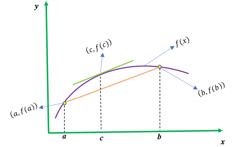
Figure 2.1: Geometric interpretation of mean value theorem
2.1.2 Application of Mean Value Theorem
Mean value theorem is the relationship between the derivative of a function and increasing or decreasing nature of function. Below are few important results.
Let the function be \(f(x)\) such that it is continuous in interval \(\left\lbrack a,b \right\rbrack\) and differentiable on interval \(\left( a,b \right)\), then \(f'(x)\) = 0, \(x\) ∈ \(\left( a,b \right)\), then \(f(x)\) is constant in \(\left\lbrack a,b \right\rbrack\)
Let \(f(x)\) and \(g(x)\) be two functions such that, \(f(x)\) and \(g(x)\) are continuous in interval \(\left\lbrack a,b \right\rbrack\) and differentiable on interval \(\left( a,b \right)\), then if, \(f'(x)\) = \(g'(x)\), x ∈ \(\left( a,b \right)\), then \(f(x)\) – \(g(x)\) is a constant in \(\left\lbrack a,b \right\rbrack\)
Strictly Increasing Function: Let the function be f such that, continuous in interval \[a, b\] and differentiable in interval (a,b). \(f^{'}\left( x \right) > 0\), \(x\) ∈ \(\left( a,b \right)\), then \(f(x)\) is strictly increasing function in \(\left\lbrack a,b \right\rbrack\)
Strictly Decreasing Function: Let the function be \(f(x)\) such that, continuous in interval \(\left\lbrack a,b \right\rbrack\) and differentiable in interval \(\left( a,b \right)\). \(f'(x)\) < 0, \(x\) ∈ \(\left( a,b \right)\), then \(f(x)\) is strictly decreasing function in \(\left\lbrack a,b \right\rbrack\).
2.1.3 Example
Verify Mean Value Theorem for the function \(f(x)\ = \ x^{2}\ –\ 4x\ –\ 3\) in the interval \(\lbrack a,\ b\rbrack\), where \(a\ =\) 1 and \(b\ =\) 4.
Solution:
Given,
\(f(x)\ = \ x^{2}\ –\ 4x\ –\ 3\)
\(f'(x)\ = \ 2x\ –\ 4\)
\(a\ = \ 1\ and\ b\ = \ 4\ (given)\)
\(f(a)\ = \ f(1)\ = \ {(1)}^{2}\ –\ 4(1)\ –\ 3\ = \ 1\ –\ 4\ –\ 3\ = \ - 6\)
\(f(b)\ = \ f(4)\ = \ {(4)}^{2}\ –\ 4(4)\ –\ 3\ = \ - 3\)
Now,
\(\frac{\lbrack f(b)\ –\ f(a)\rbrack}{\ (b\ –\ a)}\ = \ \frac{( - 3\ + \ 6)}{(4\ –\ 1)} = \frac{\ 3\ }{3} = \ 1\)
As per the mean value theorem statement, there is a point \(\text{c\ } \in \ (1,\ 4)\) such that\(\ f'(c)\ = \ \frac{\lbrack f(b)\ –\ f(a)\rbrack}{\ (b\ –\ a)}\), i.e. \(f^{'}\left( c \right) = 1\).
\(2c\ –\ 4\ = \ 1\)
\(2c\ = \ 5\)
\(c\ = \ 5/2\ \in \ (1,\ 4)\)
2.2 Rolle’s Theorem
Rolle's theorem or Rolle's lemma essentially states that any real-valued differentiable function that attains equal values at two distinct points must have at least one stationary point somewhere between them—that is, a point where the first derivative (the slope of the tangent line to the graph of the function) is zero. The theorem is named after Michel Rolle. This theorem is a special case of Lagrange’s mean value theorem.
Definition
If a function \(f(x)\) is defined in the closed interval \(\lbrack a,\ b\rbrack\ \)in such a way that it satisfies the following conditions.
The function \(f(x)\ \)is continuous over the interval \(\left\lbrack a,b \right\rbrack\).
The function \(f(x)\ \)is differentiable over the interval \(\left( a,b \right)\).
Now if \(f(a)\ \)= \(f(b)\), then there exists at least one value of \(x\), let us assume this value to be \(c\), where \(c\) ∈ \(\left( a,b \right)\) in such a way that \(f‘(c)\ = \ 0\) .
Precisely, if a function is continuous on the closed interval \(\lbrack a,\ b\rbrack\) and differentiable on the open interval \((a,\ b)\) then there exists a point \(x\ = \ c\) in \((a,\ b)\) such that \(f'(c)\ = \ 0\)
2.2.1 Geometric interpretation
In the given figure 2.2, the curve \(y\ = \ f(x)\) is continuous between \(x\ = \ a\) and \(x\ = \ b\) and at every point, within the interval, it is possible to draw a tangent and ordinates corresponding to the abscissa and are equal then there exists at least one tangent to the curve which is parallel to the \(x\)-axis.
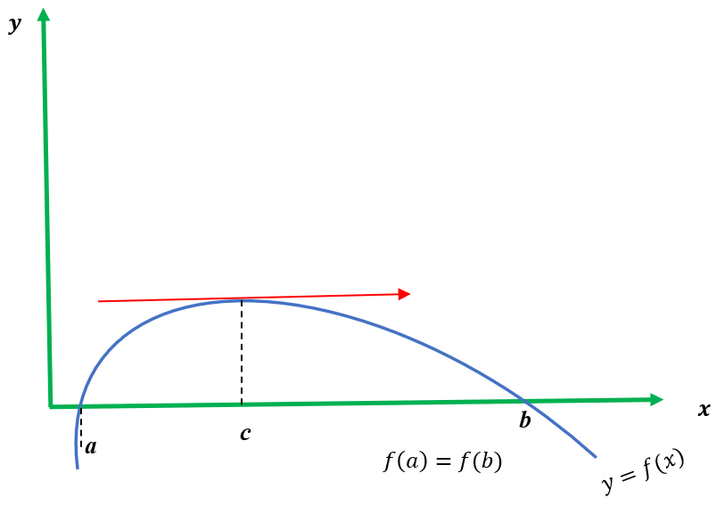
Figure 2.2: Geometric interpretation of Rolle’s theorem
2.2.2 Example
Verify Rolle’s theorem for the function \(y\ = \ x^{2}\ + \ 2\) , \(a\ = \ –2\) and \(b\ = \ 2.\)
Solution:
From the definition of Rolle’s theorem, the function \(y\ = \ x^{2}\ + \ 2\) is continuous in \(\lbrack –\ 2,\ 2\rbrack\) and differentiable in \(\left( –\ 2,\ 2 \right).\)
From the given,
\(f(x)\ = \ x^{2} + \ 2\)
\(f( - 2)\ = \ ( - 2)^{2}\ + \ 2\ = \ 4\ + \ 2\ = \ 6\)
\(f(2)\ = \ (2)^{2}\ + \ 2\ = \ 4\ + \ 2 = \ 6\)
Thus, \(f(–\ 2)\ = \ f(\ 2)\ = \ 6\)
Hence, the value of \(f(x)\ \)at –2 and 2 coincide.
Now, \(f'(x)\ = \ 2x\ \)
Rolle’s theorem states that there is a point \(\text{c\ } \in \ (–\ 2,\ 2)\) such that \(f'(c)\ = \ 0.\ \)
At \(c\ = \ 0,\ f'(c)\ = \ 2(0)\ = \ 0\), where \(c\ = \ 0\ \in \ (–\ 2,\ 2)\)
Algebraically, this theorem tells us that if \(f(x)\) is representing a polynomial function in \(x\) and the two roots of the equation \(f(x)\ = \ 0\) are \(x\ = \ a\) and \(x\ = \ b\), then there exists at least one root of the equation \(f‘(x)\ = \ 0\ \)lying between these values. The converse of Rolle’s theorem is not true