Translate an agricultural question into a null and alternative hypothesis, select an independent or paired t-test, analyze a contingency table, and interpret effect sizes, intervals, and p-values.
11.2 From description to inference
Descriptive statistics summarize observed data. Inference uses a sampling or randomization model to reason about an unobserved population or treatment effect. The experimental unit is the smallest unit independently assigned a treatment. Five leaves measured on each of four treated plants do not create twenty independently treated plants.
A null hypothesis specifies a reference claim, such as zero difference in population means. A test statistic measures discrepancy from that claim relative to sampling variation. A p-value is the probability, under the null model and its assumptions, of a test statistic at least as extreme as the observed one. It is not the probability that the null hypothesis is true, nor the probability that a result will replicate.
Choose the significance level and primary question before inspecting outcomes. Report an estimated effect and an interval alongside the p-value. Statistical significance does not imply agricultural or economic importance. Failure to reject is not proof of equality.
11.3 Worked example: uncertainty in a mean
For independent observations with unknown population variance, a two-sided confidence interval for a population mean is
The critical value comes from a Student t distribution with n - 1 degrees of freedom. It is larger than the normal critical value when the sample is small, reflecting additional uncertainty in estimating the variance.
y <-c(4.2, 4.8, 5.1, 4.5)se <-sd(y) /sqrt(length(y))critical <-qt(.975, df =length(y) -1)c(mean =mean(y), se = se, lower =mean(y) - critical * se,upper =mean(y) + critical * se)
     mean        se     lower     upper
4.6500000 0.1936492 4.0337219 5.2662781
The interval is approximately 4.03 to 5.27 t/ha. It estimates a population mean under the sampling assumptions; it is not an interval containing 95% of individual plot yields. Four conveniently selected plots would not justify population inference merely because the formula can be evaluated.
For a two-sample comparison, the same principle estimates a difference and its standard error. Welch’s method estimates variance contributions separately and adjusts the reference degrees of freedom. For a paired comparison, apply the one-sample idea to within-pair differences.
11.4 One-sample and two-sample t-tests
PlantGrowth is a real dataset supplied with R containing dry-weight measurements for a control and two treatment groups. The documentation does not identify the treatments as fertilizer rates, so do not invent that interpretation.
control <-subset(PlantGrowth, group =="ctrl")$weightt.test(control, mu =5)
    One Sample t-test

data:  control
t = 0.17355, df = 9, p-value = 0.8661
alternative hypothesis: true mean is not equal to 5
95 percent confidence interval:
 4.614882 5.449118
sample estimates:
mean of x
    5.032
The one-sample example asks whether the population mean control weight differs from 5 in the dataset’s measurement units. The reference value is an illustrative benchmark, not a verified agronomic target.
For two independent groups, Welch’s t-test allows unequal population variances and is R’s default. Define the contrast order explicitly so the sign of the estimate is unambiguous.
treated <-subset(PlantGrowth, group =="trt2")$weightwelch <-t.test(treated, control, alternative ="two.sided")welch
    Welch Two Sample t-test

data:  treated and control
t = 2.134, df = 16.786, p-value = 0.0479
alternative hypothesis: true difference in means is not equal to 0
95 percent confidence interval:
 0.00512787 0.98287213
sample estimates:
mean of x mean of y
    5.526     5.032
The t-test assumes independent observations and appropriate conditions for inference on the mean. With small samples, inspect strong skewness and outliers; normality of model errors matters more than the appearance of a pooled distribution. Welch’s test relaxes equal variance, not independence. Do not choose a one-sided alternative after seeing the sign of the difference.
11.5 Paired observations
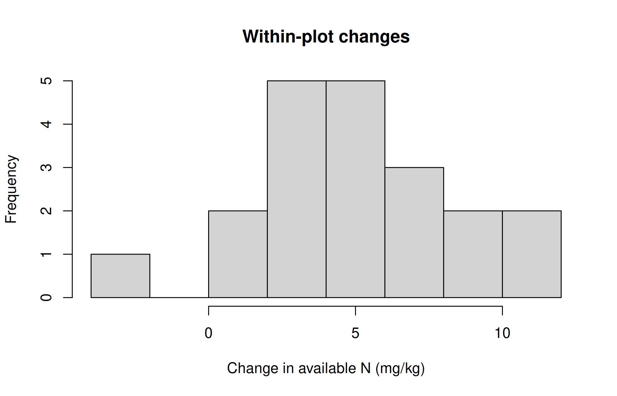
A paired design compares linked observations, such as before-and-after measurements on the same plots. The analysis uses within-pair differences. It differs from treating the two measurements as unrelated groups.
paired <-read.csv("data/paired_soil.csv")stopifnot(!anyDuplicated(paired$plot_id), complete.cases(paired))paired$change <- paired$after_mg_kg - paired$before_mg_kghist(paired$change, xlab ="Change in available N (mg/kg)", main ="Within-plot changes")
    Paired t-test

data:  paired$after_mg_kg and paired$before_mg_kg
t = 6.5908, df = 19, p-value = 2.62e-06
alternative hypothesis: true mean difference is not equal to 0
95 percent confidence interval:
 3.541818 6.838182
sample estimates:
mean difference
           5.19
Pairs must be correctly matched; the differences should be independent across pairs. Normality is assessed for differences, not separately for before and after values. Without an untreated comparison, a before–after increase may reflect time or seasonal effects as well as management.
11.6 Chi-square tests for pest observations
A contingency table cross-classifies counts. In the simulated pest dataset, each independently treated plot contributes one yes/no infestation status at a specified assessment date. The table is not composed of repeated observations of the same insects.
pest <-read.csv("data/pest.csv")tab <-with(pest, table(treatment, infested))tab
         infested
treatment No Yes
  Control 20  40
  IPM     46  14
proportions(tab, margin =1)
         infested
treatment        No       Yes
  Control 0.3333333 0.6666667
  IPM     0.7666667 0.2333333
The null hypothesis is independence between treatment and infestation status. Expected counts are calculated under independence, not taken from observed counts. The chi-square approximation needs adequate expected frequencies and independent units. For sparse 2-by-2 tables, Fisher’s exact test is often suitable; it does not fix dependence or poor sampling.
fisher.test(tab)
    Fisher's Exact Test for Count Data

data:  tab
p-value = 3.183e-06
alternative hypothesis: true odds ratio is not equal to 1
95 percent confidence interval:
 0.06268524 0.36395035
sample estimates:
odds ratio
 0.1549382
Report infestation proportions and their contrast, not only a test result. Because this example is simulated, no real pest-control efficacy claim follows. In a clustered field survey, observations from the same field may require a model that accounts for clustering.
11.7 What Welch’s test calculates
Suppose two independent groups have sample means \(\bar{x}_1\) and \(\bar{x}_2\), sample variances \(s_1^2\) and \(s_2^2\), and sizes \(n_1\) and \(n_2\). Under a null difference of zero, Welch’s statistic is
The numerator is the estimated effect. The denominator is its estimated standard error. A difference can therefore produce a larger absolute t-statistic when within-group variation is lower or sample sizes are larger. This does not make the underlying biological difference larger; it changes its precision relative to noise.
The degrees of freedom need not be an integer. They account approximately for uncertainty in the two variance estimates. In contrast, the pooled-variance t-test assumes a common population variance and estimates it using both groups. Choose the method from the design and assumptions rather than selecting whichever one gives a smaller p-value.
11.8 Reading a contingency table cell by cell
Under independence, a contingency table’s expected count is its row total multiplied by its column total and divided by the grand total. For example, if there are 60 control plots and 50 infested plots among 120 plots overall, independence predicts 60 * 50 / 120 = 25 infested control plots. The observed number need not be 25; the difference contributes to the test statistic.
Squaring prevents positive and negative discrepancies from cancelling. Dividing by the expected count scales discrepancies relative to their expected magnitude. In a two-by-two table the independence test has one degree of freedom. In a general r-by-c table it has (r - 1)(c - 1) degrees of freedom when the usual assumptions apply.
A test of association does not by itself give the direction or size of an efficacy effect. Inspect row proportions and define a contrast such as risk difference or risk ratio. If treatments were randomized to independent plots, the contrast can support a treatment interpretation within the experiment’s scope. If farmers chose their treatments, management and pest risk may already differ before treatment.
11.9 Type I error, Type II error, and power
A Type I error rejects a true null hypothesis. The chosen significance level controls its probability under the stated test model. A Type II error fails to reject a false null. Power is the probability of rejecting the null for a specified alternative effect and design. Power is therefore not one fixed characteristic of a test: it depends on the effect size, variability, sample size, and significance level.
When planning a trial, specify the smallest difference that would matter scientifically or economically and use a defensible estimate of variation. A pilot trial can inform that estimate, but its uncertainty should be acknowledged. The following planning calculation asks for the approximate sample size per group needed to detect a difference of 0.5 t/ha when the within-group SD is 0.6 t/ha, using a two-sided two-sample test at level 0.05 and power 0.80.
planning <-power.t.test(delta = .5, sd = .6, sig.level = .05,power = .80, type ="two.sample", alternative ="two.sided")planning
     Two-sample t test power calculation

              n = 23.60472
          delta = 0.5
             sd = 0.6
      sig.level = 0.05
          power = 0.8
    alternative = two.sided

NOTE: n is number in *each* group
ceiling(planning$n)
[1] 24
This is a simple equal-size independent-group planning example. Blocking, clustering, repeated measurements, unequal allocation, and expected missingness require additional design considerations. Do not use a planning result to justify treating subsamples as independent units. Also, calculating “observed power” from the same estimated effect and p-value after a test adds little information; report the effect and interval instead.
11.10 Confidence intervals and decisions
A 95% confidence procedure has 95% coverage under repeated sampling when its assumptions hold. A particular computed interval is not a 95% probability statement about a fixed parameter in frequentist inference. Wide intervals indicate that both small and large effects may be compatible with the data. Equivalence requires a prespecified margin and an appropriate equivalence analysis; a nonsignificant t-test is insufficient.
If many outcomes or comparisons are tested, false positives become more likely. Prespecify primary comparisons, distinguish exploratory results, and use an appropriate multiplicity method when needed. The next chapter introduces Tukey comparisons after ANOVA.
11.11 Practicals 11–12 and exercises
Interpret the trt2 - ctrl estimate and its interval in words without claiming a fertilizer response.
Compare paired and unpaired tests on the soil example. Explain which matches the design.
Calculate the infestation proportion in each treatment. State the observational unit and examine expected counts.
A test returns p = 0.08. Explain why “there is no effect” is too strong.
Distinguish random sampling, random treatment assignment, and repeated subsampling.
Chapter review. Valid inference begins with design. State the contrast, quantify its size and uncertainty, and interpret the p-value conditionally on the model.
11.12 Live R laboratory
Estimate a mean difference with uncertainty
Edit the code, then select Run R. The first run downloads R into your browser and may take a little time. Copy code also lets you use this example in RStudio.
Investigate. For this simulated independent-group example, identify the estimated difference, confidence interval, and null hypothesis. A small p-value alone does not measure the practical value of a treatment.
From the browser to your practical notebook
Record the input you changed, the output you obtained, and your interpretation. These live examples use base R and work independently. The full chapter examples, including package-based analyses, remain available with copy buttons for RStudio. Browser objects last until this page is reloaded; Reset code restores the editor text. Internet access is needed on first use; long or interactive desktop tasks belong in RStudio.