Fit a one-way ANOVA, interpret sums of squares and the F-test, check residual diagnostics, use adjusted pairwise comparisons, and include blocks in a simple agricultural experiment.
12.2 Why ANOVA?
Comparing three or more means by many unadjusted t-tests increases the chance of false-positive conclusions. One-way analysis of variance begins with a global null hypothesis that all group population means are equal. Its model is
\[Y_{ij}=\mu+\tau_i+\epsilon_{ij},\]
where \(\tau_i\) represents a treatment effect and the errors are assumed independent with mean zero and common variance. Normal errors provide the classical small-sample F reference distribution. The test compares treatment mean square with residual mean square. A large F-statistic means between-group variation is large relative to unexplained within-group variation.
12.3 Worked calculation: separating sources of variation
Suppose three independently randomized groups have yields A = (3, 4, 5), B = (4, 5, 6), and C = (5, 6, 7) t/ha. The group means are 4, 5, and 6 and the grand mean is 5. For equal group size 3, treatment sum of squares is \(3[(4-5)^2+(5-5)^2+(6-5)^2]=6\). Within each group the squared deviations add to 2, giving residual sum of squares 6 across all groups.
There are 3 - 1 = 2 treatment degrees of freedom and 9 - 3 = 6 residual degrees of freedom. Treatment mean square is 6/2 = 3, residual mean square is 6/6 = 1, and the F-statistic is 3.
toy <-data.frame(group =factor(rep(c("A", "B", "C"), each =3)),yield_t_ha =c(3, 4, 5, 4, 5, 6, 5, 6, 7))summary(aov(yield_t_ha ~ group, data = toy))
            Df Sum Sq Mean Sq F value Pr(>F)
group        2      6       3       3  0.125
Residuals    6      6       1
pf(3, df1 =2, df2 =6, lower.tail =FALSE)
[1] 0.125
The p-value is 0.125. The observed means differ, but the data do not reject the global equality hypothesis at the conventional 0.05 level under this model. “Means differ in this sample” and “there is strong evidence of population differences” are distinct statements. Larger, well-designed replication may improve precision; repeating measurements of the same experimental units does not create new independent replication.
12.4 Worked example: plant dry weight
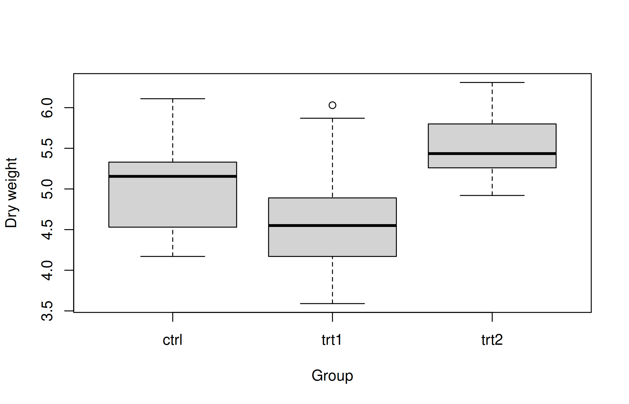
data("PlantGrowth", package ="datasets")fit <-aov(weight ~ group, data = PlantGrowth)summary(fit)
            Df Sum Sq Mean Sq F value Pr(>F)
group        2  3.766  1.8832   4.846 0.0159 *
Residuals   27 10.492  0.3886
---
Signif. codes:  0 '***' 0.001 '**' 0.01 '*' 0.05 '.' 0.1 ' ' 1
In the ANOVA table, Df gives degrees of freedom, Sum Sq partitions variation, Mean Sq divides sums of squares by degrees of freedom, and Pr(>F) gives the global p-value. Rejecting the global null indicates evidence that at least one mean differs; it does not show that every pair differs.
TukeyHSD(fit)
  Tukey multiple comparisons of means
    95% family-wise confidence level

Fit: aov(formula = weight ~ group, data = PlantGrowth)

$group
            diff        lwr       upr     p adj
trt1-ctrl -0.371 -1.0622161 0.3202161 0.3908711
trt2-ctrl  0.494 -0.1972161 1.1852161 0.1979960
trt2-trt1  0.865  0.1737839 1.5562161 0.0120064
Tukey’s method adjusts simultaneous pairwise comparisons within the specified family. Each row reports a signed difference, interval, and adjusted p-value. Read the group order carefully. Avoid reducing the entire analysis to letter groupings; report means, differences, uncertainty, and design.
12.5 Diagnose the errors, not just the raw observations
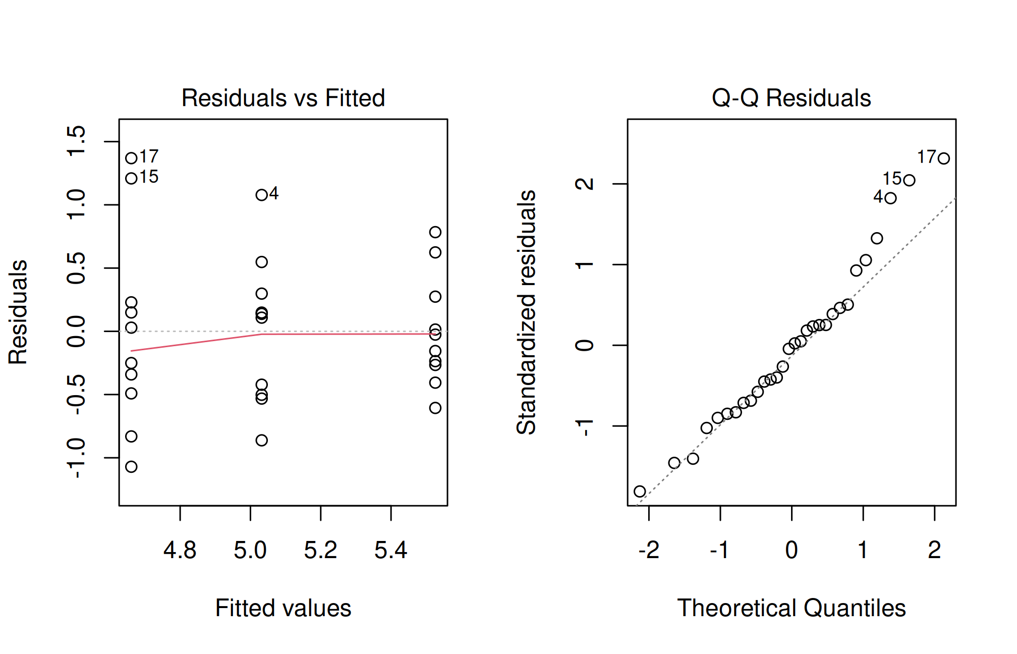
old <-par(mfrow =c(1, 2))plot(fit, which =1)plot(fit, which =2)
Residual-versus-fitted plots reveal unequal spread and patterns; normal quantile plots reveal departures from a normal error distribution. Neither a diagnostic plot nor a formal normality test can establish independence; that comes from the design. Small samples provide little information about distribution tails. A single normality p-value should not act as an automatic gatekeeper.
If variances differ substantially, Welch’s one-way test is an alternative for independent groups:
oneway.test(weight ~ group, data = PlantGrowth, var.equal =FALSE)
    One-way analysis of means (not assuming equal variances)

data:  weight and group
F = 5.181, num df = 2.000, denom df = 17.128, p-value = 0.01739
Welch’s test does not use the ordinary equal-variance ANOVA error term. Do not follow it automatically with classical TukeyHSD(); choose pairwise methods compatible with unequal variances if needed.
12.6 Blocking in agricultural experiments
Field fertility may vary across space. A randomized complete block design assigns every treatment once within each block, with randomization within blocks. The additive model includes both treatment and block:
\[Y_{ij}=\mu+\tau_i+\beta_j+\epsilon_{ij}.\]
The supplied simulated rcbd.csv has six blocks and three treatment plots per block. It differs from the larger crop dataset, which also includes variety and replicate plots. Do not analyze that factorial dataset as though it were this simple RCBD.
Representing block as a factor avoids imposing a linear trend in arbitrary block numbers. With one plot per treatment in each block, a separate treatment-by-block interaction cannot be estimated independently of residual error. The additive model assumes that interaction is negligible for its intended interpretation. Inference beyond the observed blocks and more complex designs may require mixed models.
Ignoring blocks can waste precision and misrepresent the design. Conversely, adding terms without understanding randomization does not create a valid analysis. The default ANOVA sums of squares are sequential; in unbalanced designs, term order and the exact hypothesis require attention. The balanced examples here keep that issue visible without treating advanced factorial analysis as a one-line extension.
12.7 Reading treatment comparisons in their experimental context
Let us distinguish three quantities that are often placed in the same results table: a treatment mean, the standard deviation of individual plots in that treatment, and the standard error of an estimated treatment contrast. The mean describes a central response. The SD describes plot variation. The contrast’s standard error depends on the model and design, including the number of replicates and any blocking adjustment.
For a balanced independent one-way design with r plots per treatment and residual mean square MSE, the standard error of a difference between two treatment means is \(\sqrt{2\,MSE/r}\). In a balanced additive RCBD the analogous contrast uses the residual variance after accounting for blocks. This is why treatment comparisons should use the appropriate model’s error term rather than the spread of the three treatment means.
This standard error does not itself adjust for examining all treatment pairs. Multiplicity adjustments change the critical comparison or interval construction. A planned comparison identified before data collection may ask a more focused question than all pairwise comparisons, such as average response under two management treatments versus the control. Its weights and intended hypothesis should be stated explicitly.
12.8 A factorial extension: treatment and variety
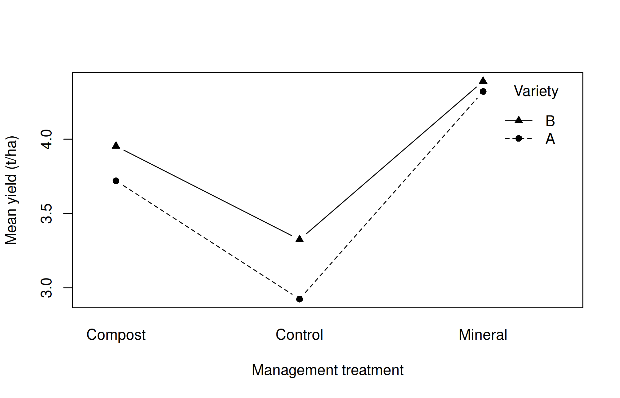
In agricultural research, two factors may be applied together. A factorial experiment observes combinations of their levels. Here the larger simulated crop dataset contains three management treatments and two varieties in each of five blocks, with two independently measured plot replicates for each combination. This allows us to illustrate a treatment-by-variety interaction.
The expression treatment * variety expands to both main effects and their interaction. An interaction means that the difference between varieties depends on management treatment, or equivalently that a management contrast depends on variety. A single overall treatment difference can then conceal an important pattern. Nonparallel sample lines suggest an interaction to examine, but sampling variation can also make them nonparallel.
If interaction is important scientifically, report comparisons within relevant levels with an appropriate simultaneous procedure. Do not interpret a nonsignificant interaction as proof that responses are identical across varieties. Likewise, do not remove an interaction solely to make a main effect significant. Consider the question, precision, and experimental design.
The factorial example assumes both factors were randomized at the plot level within blocks. If irrigation is applied to whole field sections and variety to smaller subplots, the error structure changes. A split-plot experiment needs a split-plot analysis; entering the same factor names into an ordinary one-error ANOVA is not sufficient.
12.9 Reporting an ANOVA analysis
A useful report identifies the design, factor levels, independent replication, model, and any exclusions before presenting the table. Report treatment estimates with units, the global test and relevant degrees of freedom, the method used for comparisons, and the main diagnostic findings. An agronomic interpretation should explain the size of a response, not merely its statistical label.
For example, a small positive difference with a wide interval may justify a larger experiment rather than a recommendation. A precisely estimated increase may still be uneconomic if the treatment is costly. A trial at one site and season does not establish performance under all environments. These are not flaws that another p-value can repair; they define the scope of the evidence.
12.10 Practical 13 and exercises
Explain the global null in PlantGrowth and identify residual degrees of freedom.
Interpret one Tukey interval and its adjusted p-value.
Fit the RCBD model with and without block. Compare residual mean squares and explain why the design supports including block.
Explain why an ANOVA on three treatment means alone cannot estimate plot-to-plot error correctly.
Propose a suitable randomization scheme for a three-treatment experiment on a field with a fertility gradient.
Chapter review. ANOVA partitions variation according to a model. The model should follow randomization, and a global comparison must be distinguished from individual treatment contrasts.
12.11 Live R laboratory
Compare three treatment means
Edit the code, then select Run R. The first run downloads R into your browser and may take a little time. Copy code also lets you use this example in RStudio.
Investigate. The omnibus F test and Tukey comparisons answer different questions. Consult the chapter for randomization, independence, residual checks, and how an ANOVA model changes for blocked designs.
From the browser to your practical notebook
Record the input you changed, the output you obtained, and your interpretation. These live examples use base R and work independently. The full chapter examples, including package-based analyses, remain available with copy buttons for RStudio. Browser objects last until this page is reloaded; Reset code restores the editor text. Internet access is needed on first use; long or interactive desktop tasks belong in RStudio.