13Correlation and regression for agricultural prediction
13.1 Learning outcomes
Distinguish Pearson and Spearman correlation, interpret simple and multiple regression coefficients, check model assumptions and influential observations, and evaluate prediction on held-out observations.
13.2 Association is not a treatment effect
Pearson’s correlation measures the strength and direction of a linear relationship between quantitative variables. Spearman’s correlation applies Pearson’s idea to ranks and describes monotonic association. Neither establishes causation, and a value near zero need not imply the absence of a nonlinear relationship. Both can be distorted by pooling unlike groups or by dependence among observations.
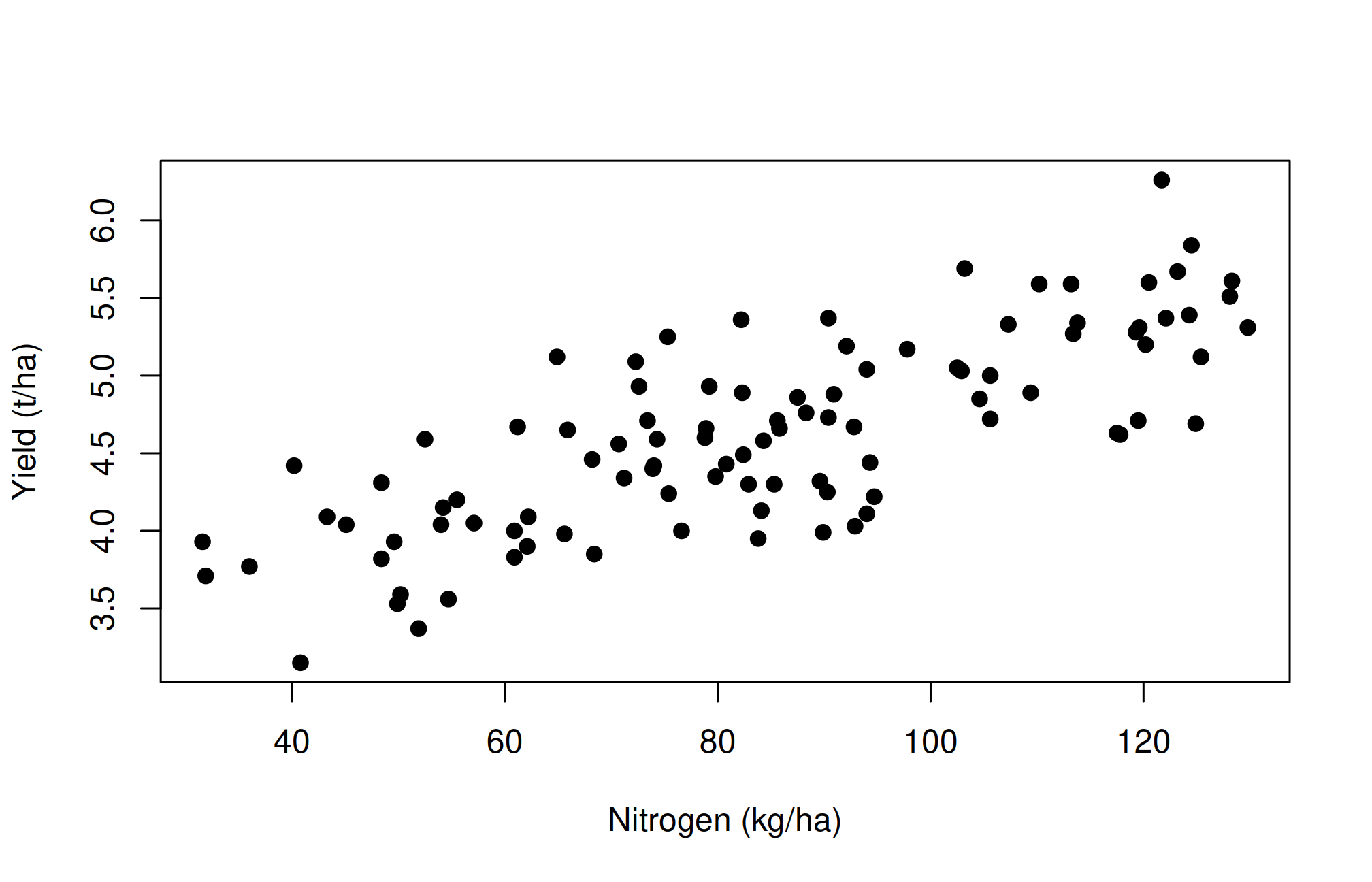
The simulated farm_yield.csv contains 100 independent teaching records with nitrogen application, seasonal rainfall, and yield. It is constructed for a regression lesson and is not evidence for a real fertilizer recommendation.
    Spearman's rank correlation rho

data:  farm$nitrogen_kg_ha and farm$yield_t_ha
S = 40283, p-value < 2.2e-16
alternative hypothesis: true rho is not equal to 0
sample estimates:
      rho
0.7582784
Inspect scatter plots before interpreting a correlation coefficient. Pearson’s usual test assumes independent pairs and a suitable bivariate sampling model; ranks do not fix clustering or confounding. Spearman’s test uses an approximation here because rounded measurements can create ties.
13.3 Simple linear regression
The model \(Y_i=\beta_0+\beta_1X_i+\epsilon_i\) describes a conditional mean response. The intercept is the predicted mean when \(X=0\); the slope is a change in mean response per unit increase in \(X\). Least squares minimizes squared residuals. The regression direction matters: a model predicting yield from nitrogen is not interchangeable with one predicting nitrogen from yield.
simple <-lm(yield_t_ha ~ nitrogen_kg_ha, data = farm)summary(simple)
Call:
lm(formula = yield_t_ha ~ nitrogen_kg_ha, data = farm)

Residuals:
     Min       1Q   Median       3Q      Max
-0.74926 -0.29294  0.02507  0.24883  0.95320

Coefficients:
               Estimate Std. Error t value Pr(>|t|)
(Intercept)    3.077606   0.135654   22.69   <2e-16 ***
nitrogen_kg_ha 0.018317   0.001539   11.90   <2e-16 ***
---
Signif. codes:  0 '***' 0.001 '**' 0.01 '*' 0.05 '.' 0.1 ' ' 1

Residual standard error: 0.3957 on 98 degrees of freedom
Multiple R-squared:  0.591, Adjusted R-squared:  0.5868
F-statistic: 141.6 on 1 and 98 DF,  p-value: < 2.2e-16
The slope has units t/ha of yield per kg/ha of applied nitrogen. Its estimate is an association in these data, conditional on the specified model. If zero nitrogen lies outside the observed range, the intercept is an extrapolation and need not have a useful agronomic interpretation.
13.4 Worked calculation: what least squares estimates
For a simple regression with an intercept, the estimated slope is
The slope is undefined when every predictor value is identical: the denominator is zero. A range of predictor values is necessary to estimate a relationship. The calculation below verifies the coefficients from lm() rather than treating its output as a black box.
Residuals are observed minus fitted responses. With an intercept, least squares makes their sum approximately zero. This algebraic property does not show that their errors are independent or normally distributed. Those require design knowledge and diagnostics.
13.5 Multiple regression and conditional coefficients
multiple <-lm(yield_t_ha ~ nitrogen_kg_ha + rainfall_mm, data = farm)summary(multiple)
Call:
lm(formula = yield_t_ha ~ nitrogen_kg_ha + rainfall_mm, data = farm)

Residuals:
     Min       1Q   Median       3Q      Max
-0.75803 -0.26042  0.02216  0.22680  0.66787

Coefficients:
                Estimate Std. Error t value Pr(>|t|)
(Intercept)    1.9792857  0.2317298   8.541 1.87e-13 ***
nitrogen_kg_ha 0.0179861  0.0013508  13.315  < 2e-16 ***
rainfall_mm    0.0017326  0.0003137   5.522 2.80e-07 ***
---
Signif. codes:  0 '***' 0.001 '**' 0.01 '*' 0.05 '.' 0.1 ' ' 1

Residual standard error: 0.3469 on 97 degrees of freedom
Multiple R-squared:  0.6888,    Adjusted R-squared:  0.6824
F-statistic: 107.4 on 2 and 97 DF,  p-value: < 2.2e-16
The nitrogen coefficient now describes a change while rainfall is held fixed in the model. It may differ from the simple-regression coefficient because the models ask different questions. Omitted confounders, measurement error, and nonlinearity can still bias interpretation. Adding predictors raises ordinary \(R^2\) even if they contribute little; high \(R^2\) does not establish causality or reliable future prediction.
Strongly correlated predictors make separate coefficients unstable. In the crop trial, treatment and applied nitrogen are closely linked, so including both without thought can make individual effects hard to interpret. Select predictors using scientific reasoning, design, and an evaluation plan rather than repeated p-value searches.
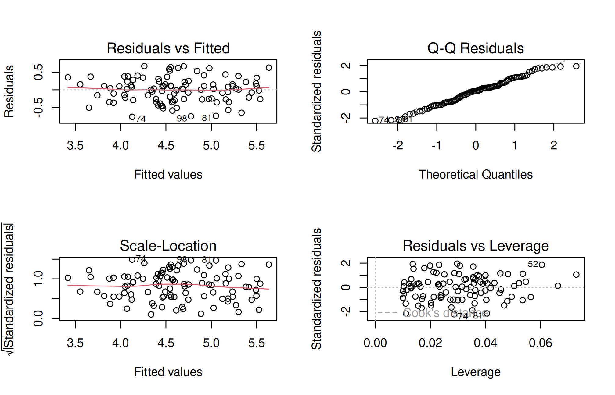
The residual-versus-fitted plot checks mean structure, the Q–Q plot checks the error distribution, the scale-location plot checks spread, and leverage/influence diagnostics identify observations that can strongly affect estimates. Check influential records against source information; do not delete them merely to improve fit. Classical t-tests and intervals need assumptions about errors, including independence and constant variance. Normality concerns the errors for small-sample inference, not every predictor’s marginal distribution.
13.7 Categorical predictors and reference levels
Regression can include categorical variables through indicator coding. A two-variety example illustrates this without requiring the varieties to be interpreted as numeric doses. The reference level determines the intercept’s meaning, while the fitted mean for each observation remains unchanged under a consistent recoding.
The varietyB coefficient compares B with A conditional on the other terms in this additive model. It assumes a common variety difference across treatments. The preceding ANOVA chapter explains how a treatment-by-variety interaction relaxes that assumption. ANOVA and regression are connected expressions of linear modelling, rather than unrelated procedures selected solely by the appearance of a response column.
13.8 Residual standard error and explained variation
The residual sum of squares measures unexplained squared deviations after fitting. Dividing by residual degrees of freedom and taking a square root gives the residual standard error, in yield units. \(R^2\) compares residual sum of squares with the total sum of squares around the observed mean:
An in-sample \(R^2\) describes fit to the observed response variation under that model. It is not the percentage probability that a prediction is correct. A narrow predictor range can produce a low \(R^2\) even when a small slope is estimated usefully; a common time trend can produce a high \(R^2\) for an unsuitable causal interpretation. Compare models in relation to their purpose and predictor domain.
13.9 Nonlinearity and an apparent fertilizer optimum
Crop response to a nutrient may increase initially and then approach a plateau or decline. A straight line over a restricted range can approximate part of that response without defining a biological optimum. A quadratic model adds a squared predictor term. In R formulas, write I(x^2) so the power is interpreted arithmetically.
Call:
lm(formula = yield_t_ha ~ nitrogen_kg_ha + I(nitrogen_kg_ha^2) +
    rainfall_mm, data = farm)

Residuals:
     Min       1Q   Median       3Q      Max
-0.76092 -0.25807  0.02466  0.22923  0.67272

Coefficients:
                     Estimate Std. Error t value Pr(>|t|)
(Intercept)         2.034e+00  4.050e-01   5.021 2.37e-06 ***
nitrogen_kg_ha      1.660e-02  8.536e-03   1.945   0.0547 .
I(nitrogen_kg_ha^2) 8.248e-06  5.019e-05   0.164   0.8698
rainfall_mm         1.730e-03  3.158e-04   5.479 3.44e-07 ***
---
Signif. codes:  0 '***' 0.001 '**' 0.01 '*' 0.05 '.' 0.1 ' ' 1

Residual standard error: 0.3487 on 96 degrees of freedom
Multiple R-squared:  0.6889,    Adjusted R-squared:  0.6792
F-statistic: 70.87 on 3 and 96 DF,  p-value: < 2.2e-16
For a concave quadratic \(a+bN+cN^2\) with \(c<0\), its mathematical maximum occurs at \(-b/(2c)\). If c is positive, the stationary point is a minimum, not an optimum. Even a concave fitted curve may place its maximum outside the observed nitrogen range, where it is unsupported extrapolation. The supplied simulation is generated with a linear mean response, so a quadratic term should not be presented as discovering a true fertilizer optimum.
An economic optimum additionally depends on crop price, input cost, and an appropriate response function. A fitted yield curve alone cannot supply those missing quantities. A defensible recommendation also needs replicated evidence across relevant environments and an assessment of uncertainty. In this introductory course, use nonlinear patterns to motivate questions and model checks before offering recommendations.
         method      RMSE       MAE
1    Regression 0.3892038 0.3225455
2 Training mean 0.6895416 0.5703840
A confidence interval concerns the mean response at the specified predictors; a prediction interval includes variation in a new observation and is wider. Both rely on the model. Avoid extrapolation outside the training range and consider combinations of predictors that may be unusual even when each is individually within range.
A random holdout is suitable for these independent simulated records. For repeated farms, spatial clusters, or time series, split by group, location, or time as appropriate. Fit preprocessing steps using training data only. One split gives an unstable estimate, so cross-validation may be needed for serious model comparison. The test set should not become another training set through repeated tuning.
13.11 Practical 14 and exercises
Compare Pearson and Spearman coefficients and explain their target relationships.
Interpret the rainfall coefficient and its units. Why is it not automatically a causal rainfall effect?
Compare simple and multiple nitrogen slopes. Explain what changes in their interpretation.
Compare a confidence and prediction interval for the same new record.
Evaluate the held-out model against the training-mean baseline. Identify a realistic setting where a random row split would be inappropriate.
Chapter review. Correlation describes association; regression specifies a conditional response; prediction requires separate evaluation. Design and domain knowledge remain necessary for causal interpretation.
13.12 Live R laboratory
Fit and interpret a yield model
Edit the code, then select Run R. The first run downloads R into your browser and may take a little time. Copy code also lets you use this example in RStudio.
Investigate. Interpret the slope with units and distinguish a prediction interval for a new observation from a confidence interval for the mean. Do not extrapolate this simulated linear response to arbitrary doses.
From the browser to your practical notebook
Record the input you changed, the output you obtained, and your interpretation. These live examples use base R and work independently. The full chapter examples, including package-based analyses, remain available with copy buttons for RStudio. Browser objects last until this page is reloaded; Reset code restores the editor text. Internet access is needed on first use; long or interactive desktop tasks belong in RStudio.