3 Analysis of Variance (ANOVA)
Consider an example where three chemical fertilizers A, B, C are tested on potted plants. Experimenter would like to identify, which among the fertilizer among A, B and C gives the highest yield. Potted plants are maintained in the same way; so that experimental conditions are homogenous. Now after collecting yield data from the plants, you can observe a variance i.e., the yield values are not same. Here, this variation is caused by the treatment and experimental error. So, the total observed variance = variance due to treatments + variance due to error. So, in this example treatment and error can be considered as the source of variation in the data. Basically, any experiment you perform is a sample based on which you make generalization about the population. Now, based on your experiment you want to test whether the means of treatment A, B and C are significantly different considering that the observed difference is not by chance taking in to account experimental error variance.
Analysis of variance (ANOVA) is a statistical procedure used to analyze the differences among means, where the observed total variance is partitioned into components attributable to different sources of variation. The logic behind is simple, if much of the variation comes from the treatment, it is more likely that the mean of treatments is different. This variation is compared with the experimental error variance, larger the ratio of treatment variance to error variance, the more likely that the groups have different means. The term "analysis of variance" originates from how the analysis uses variances to determine whether the means are different. ANOVA works by comparing the variance of treatments (between group variance) to the error variance (within group variance).
In short ANOVA is a statistical hypothesis test that determines whether the means of at least two populations are different. ANOVA was developed by the statistician Sir Ronald A. Fisher.
3.1 Null hypothesis in ANOVA
Null hypothesis in ANOVA is that population means are equal, which is denoted as H0: µ1 = µ2 =µ3 = …., = µk . Alternate hypothesis is that atleast a pair of treatment are not equal, H1: µi ≠ µj, where i ≠ j; i, j = 1,2, …, k. Where µ1, µ2, µ3, …, µk are k population means
3.2 Degrees of freedom
Before proceeding, it is important to understand the concept of degrees of freedom. Degrees of freedom can be defined as the number of independent observations that are free to vary.
Consider a simple example, you have 7 hats and you want to wear a different hat every day of the week. On the first day, you can wear any of the 7 hats. On the second day, you can choose from the 6 remaining hats, on day 3 you can choose from 5 hats, and so on. When day 6 rolls around, you still have a choice between 2 hats that you haven’t worn yet that week. But after you choose your hat for day 6, you have no choice for the hat that you wear on Day 7. You must wear the one remaining hat. You had 7-1 = 6 days of “hat” freedom—in which the hat you wore could vary!
Degrees of freedom can also be defined as the number of independent values, which were included into calculation of an estimate. An estimate is a single number that expresses some property of a population from a sample. It can be mean, median, standard deviation, or variance that is calculated from a sample. And there are independent values (or observations) that went into formula calculation. The quantity of these values is called “degrees of freedom.”
Consider three observations 6, x and 9. Here x is unknown and suppose we know the mean is 6. Then we can say x is exactly equal to 3, because mean is 6. Here two values are free to vary but the third value depends on other two under the constraint that their mean should be 6. i.e. if other two values are changed third value will also change.
Now consider the height of 7 students
164, 173, 158, 179, 168, 187, 167.
Mean: 170.85
We can find standard deviation using two formulas
SD= \(\frac{\sum_{}^{}\left( x_{i} - \overline{x} \right)^{2}}{n}\), where n is the number of observations
Here SD = 9
SD= \(\frac{\sum_{}^{}\left( x_{i} - \overline{x} \right)^{2}}{n - 1}\), where n-1 is the degrees of freedom
Here SD = 9.72
It is easy to notice that when we divide by degrees of freedom, we make our estimate of standard deviation greater than if we were diving only by sample size. But why do we need to make it greater? As we’ve already calculated the mean, we don’t have to use all the data in order to estimate the standard deviation. It does not depend on each piece of information, and the last observation does not contribute to the standard deviation. So, if we don’t delete this redundant data, then we underestimate the standard deviation of population from sample data. So here using the degrees of freedom in the denominator provides an unbiased estimate of population standard deviation.
Degrees of freedom also define the probability distributions for the test statistics of various hypothesis tests. For example, hypothesis tests use the t-distribution, F-distribution, and the chi-square distribution to determine statistical significance. Each of these probability distributions is a family of distributions where the DF define the shape. Hypothesis tests use these distributions to make decisions on null hypothesis.
3.3 Mean squares
The sum of squares is the sum of the square of difference of each observation from mean. That is Sum of squares =\(\sum_{i = 1}^{n}\left( x_{i} - \overline{x} \right)^{2}\). Where, i =1, 2, …, n, mean \(\overline{x} = \frac{\sum_{i = 1}^{n}x_{i}}{n}\). Sum of squares generates a measure of variability. In One-way ANOVA we calculate sum of squares of all observation to get measure of total variability along with within group and between group sum of squares, that gives idea on with in (error) and between group (between treatments) variability respectively. Mean sum of squares or mean squares are obtained by dividing sum of squares by corresponding degrees of freedom. Mean square provides unbiassed estimate of variance. For example, in ANOVA error mean square (MSE) given by \(\frac{\text{with in group sum of squares}}{\text{error degrees of freedom}}\) provides unbiased estimate of error variance
3.4 Test Statistic F
Any function of sample values is known as a statistic. For example, sample mean, sample variance, sum of all sample values are statistic, because these are all some functions of sample values. If a statistic is used to test a hypothesis, then it is known as test statistic. Examples of test statistic are t, F, χ2 etc. The test statistic used in ANOVA is F.
F-statistic is the ratio of two variances and it was named after Sir Ronald A. Fisher. It is proved that when null hypothesis H0: µ1 = µ2 =µ3 = …., = µk is true the ratio of mean square treatment and mean square error follows F distribution.The F distribution is a right-skewed distribution. In general, if your calculated F value in ANOVA is larger than your F critical value, you can reject the null hypothesis.
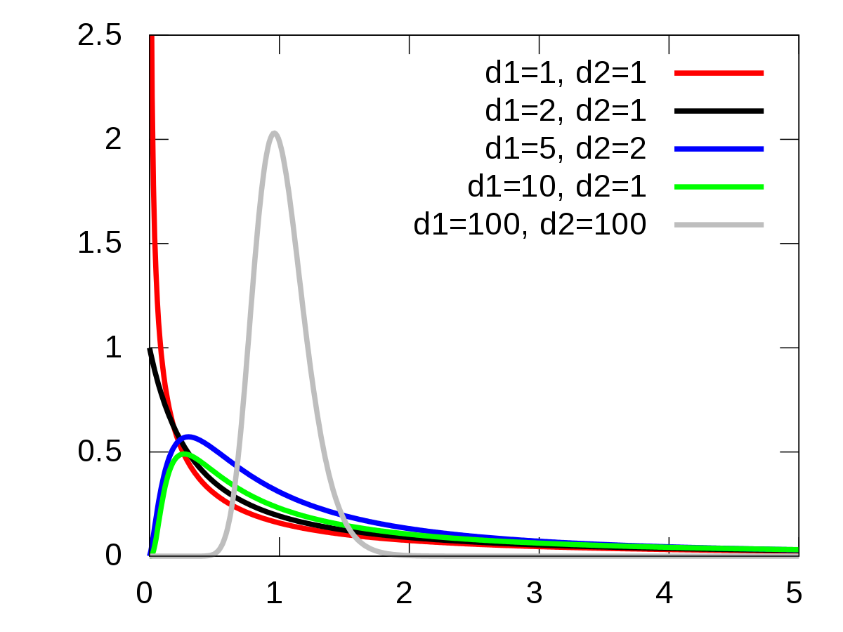
Figure 3.1: Distribution F under different degrees of freedom
3.5 Assumptions of ANOVA
Observations under each treatment group is drawn randomly from a normally distributed population
All the populations from which observations are drawn have a common variance :- Homogeneity of variance
All the samples are drawn independently of each other
Treatment and environmental effects are additive
As a result of above assumptions. The experimental errors are independent and identically distributed (iid) with a Normal distribution of mean 0 and variance σ2. In other word we can say \(e_{i}\) \(\sim iid\ N(0,\sigma^{2})\).
3.6 Types of ANOVA
Based on the model used and sources of variation studied ANOVA can be classified into following types
- One-way ANOVA
- Two-way ANOVA
- m-way ANOVA
3.6.1 One-way ANOVA
The simplest type of analysis of variance is known as one way analysis of variance, in which only one source of variation or factor of interest is controlled and its effect on the elementary units is observed. See the example in section 3.7.1 is an example where one-way ANOVA can be employed. Here only one source of variation is assumed to be causing variance other than error that is field.
3.6.1.1 One -way ANOVA model {oneway}
\[Y_{\text{ij}} = \mu + \tau_{i} + e_{\text{ij}}\]
Where i = 1,2, …, t and j =1,2, …, r. \(Y_{\text{ij}}\) is the observed value of ith
treatment from jth replication, \(\tau_{i}\) is the effect of ith treatment. \(\mu\) is the general
effect which is common for all treatments. \(e_{\text{ij}}\) is the error
effects.\(e_{ij}\) \(\sim iid\ N(0,\sigma^{2})\)
3.6.1.2 One-way classification
Consider an experiment with v treatments with r replications each. Observations are recorded as shown below.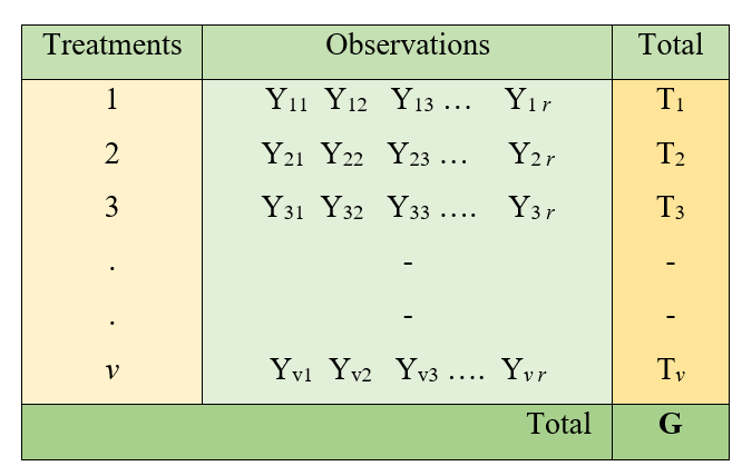
Figure 3.2: One way classification of Data
3.6.1.3 Total sum of squares partitioning
ANOVA consists of partitioning the total variation in Yij values into variation due to treatments and variation caused by uncontrolled factors (error variation). Therefore, we can write,
Variance of Yij = \(\frac{1}{n}\sum_{i = 1}^{v}\sum_{j = 1}^{r}\left( Y_{\text{ij}} - \bar{Y} \right)^{2}\)where n = v x r, overall mean \(\bar{Y} = \frac{G}{n}\)
Total Sum of Squares = \(\sum_{i = 1}^{v}\sum_{j = 1}^{r} Y_{\text{ij}}^{2} - \frac{G^{2}}{n}\); where \(\frac{G^{2}}{n}\) is known as the correction factor (C.F.).
3.6.1.3.1 Proof
= \(\sum_{i = 1}^{v}\sum_{j = 1}^{r}\left( Y_{\text{ij}} - \bar{Y} \right)^{2}\)
= \(\sum_{i = 1}^{v}\sum_{j = 1}^{r}\left( Y_{\text{ij}}^{2} - 2Y_{\text{ij}}\bar{Y} + {\bar{Y}}^{2} \right)\)
= \(\sum_{i = 1}^{v}\sum_{j = 1}^{r}\left( Y_{\text{ij}}^{2} - 2n{\bar{Y}}^{2} + n{\bar{Y}}^{2} \right)\)
= \(\sum_{i = 1}^{v}\sum_{j = 1}^{r}\left( Y_{\text{ij}}^{2} - n{\bar{Y}}^{2} \right)\)
= \(\sum_{i = 1}^{v}\sum_{j = 1}^{r} Y_{\text{ij}}^{2} - n\left( \frac{\sum_{i = 1}^{v}\sum_{j = 1} Y_{\text{ij}}}{n} \right)^{2},\)
denote \(\sum_{i = 1}^{v}\sum_{j = 1}^{r} Y_{\text{ij}} = G\)
Total Sum of Squares = \(\sum_{i = 1}^{v}\sum_{j = 1}^{r} Y_{\text{ij}}^{2} - \frac{G^{2}}{n}\)
The Total Sum of Squares is partitioned into Sum of Squares due to Treatments and Sum of Squares due to Error.
3.6.1.3.2 Proof
\[\sum_{i = 1}^{v}{\sum_{j = 1}^{r}\left( Y_{\text{ij}} - \overline{Y} \right)^{2}} = \sum_{i = 1}^{v}{\sum_{j = 1}^{r}\left( Y_{\text{ij}} - {\overline{Y}}_{i} + {\overline{Y}}_{i} - \overline{Y} \right)^{2}}\]
\[= \sum_{i = 1}^{v}{\sum_{j = 1}^{r}\left( \left( Y_{\text{ij}} - {\overline{Y}}_{i} \right)^{2} + \left( {\overline{Y}}_{i} - \overline{Y} \right)^{2} + 2\left( Y_{\text{ij}} - {\overline{Y}}_{i} \right)\left( {\overline{Y}}_{i} - \overline{Y} \right) \right)}\]
\[= \sum_{i = 1}^{v}{\sum_{j = 1}^{r}{\left( Y_{\text{ij}} - {\overline{Y}}_{i} \right)^{2} +}}\sum_{i = 1}^{v}{\sum_{j = 1}^{r}{\left( {\overline{Y}}_{i} - \overline{Y} \right)^{2} + 2\sum_{i = 1}^{v}{\sum_{j = 1}^{r}{\left( Y_{\text{ij}} - {\overline{Y}}_{i} \right)\left( {\overline{Y}}_{i} - \overline{Y} \right)}}}}\]
Let \(\left( Y_{\text{ij}} - {\overline{Y}}_{i} \right)^{2} = e_{\text{ij}}^{2}\), \(\sum_{i = 1}^{v}{\sum_{j = 1}^{r}e_{\text{ij}}} = 0\)
\[= \sum_{i = 1}^{v}{\sum_{j = 1}^{r}{{e_{\text{ij}}}^{2} +}}\sum_{i = 1}^{v}{\sum_{j = 1}^{r}{\left( {\overline{Y}}_{i} - \overline{Y} \right)^{2} + 2\sum_{i = 1}^{v}{\sum_{j = 1}^{r}{e_{\text{ij}}\left( {\overline{Y}}_{i} - \overline{Y} \right)}}}}\]
\(\sum_{i = 1}^{v}{\sum_{j = 1}^{r}{e_{\text{ij}}\left( {\overline{Y}}_{i} - \overline{Y} \right)}} = 0\), since the sum of the weighted residuals is zero, then the above equation will be
\[= \sum_{i = 1}^{v}{\sum_{j = 1}^{r}{{e_{\text{ij}}}^{2} +}}\sum_{i = 1}^{v}{\sum_{j = 1}^{r}\left( {\overline{Y}}_{i} - \overline{Y} \right)^{2}}\]
Total Sum of Square = with in group sum of square + between group sum of square
Total Sum of Square = Error sum of square + Treatment Sum of Square
3.6.1.4 Treatment sum of square
Let us denote the treatment totals as T1, T2, ….,TV i.e \({T}_{i}{\ =\ }\sum_{j = 1}^{r} Y_{\text{ij}}\) so that \(T_{1}{\ +\ }{T}_{2}{\ +\ }\text{T}_{3}{\ +\ }{T}_{n}\text{ }\text{……}{+\ }{T}_{v}{\ =\ }\sum_{i = 1}^{v}\sum_{j = 1}^{r} Y_{\text{ij}} = G\)
Treatment Sum of Squares, TSS = \(\frac{\sum_{i = 1}^{v}\text{T}\text{i}^{2}}{r} - \frac{G^{2}}{n}\).
3.6.1.5 Calculations for One-way ANOVA
Total Sum of Square (Total SS) = \(\sum_{i = 1}^{v}\sum_{j = 1}^{r} Y_{\text{ij}}^{2} - \text{C.F.}\) (square all the observations, sum it and correction factor is subtracted to get total sum of squares)
Treatment Sum of Squares (TSS) = \(\frac{\sum_{i = 1}^{v}\text{T}\text{i}^{2}}{r} - \text{C.F.}\). (square all the treatment totals, sum it and correction factor is subtracted to get treatment sum of squares )
Error Sum of Squares (ESS)= Total SS – TSS
Correction factor (C.F.) = \(\frac{G^{2}}{n}\), where \(G\) = Grand Total of all observations.
Mean sum of squares is the sum of squares divided by corresponding degrees of freedoms (d.f.).
Error degrees of freedom = Total degrees of freedom – treatment degrees of freedom.
Error d.f.= \(vr - 1 - \left( v - 1 \right) = vr - 1 - v + 1 = vr - v = v(r - 1)\)
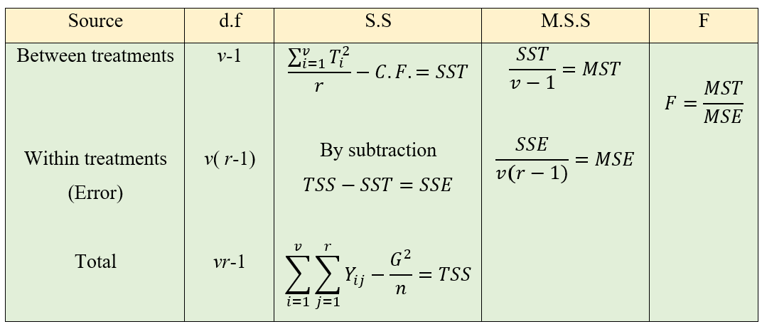
Figure 3.3: One-way ANOVA table
Here F ~ F (v-1), v(r-1)
MSE is an estimate of error variance σ2 and \(\sqrt{\frac{\text{MSE}}{r}}\) is the standard error of a treatment mean.
If your calculated F value in ANOVA is larger than your F critical value corresponding to the degrees of freedoms in the critical value table, you can reject the null hypothesis. see the section 6
3.6.1.6 Example of One-way ANOVA
The data on tiller count after transplanting were recorded from 4 hill sampling units for a fertilizer trial involving 6 treatments. Test for the significant difference between the treatments. The treatments are labeled as T1, T2, T3, T4, T5 and T6.
Data is arranged as shown below:
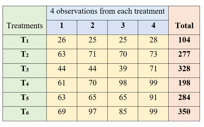
Figure 3.4: One-way classified data on tiller count
Calculation:
Here equal number of observations are taken from all treatments, so r1 = r2 = … = r6 = 4
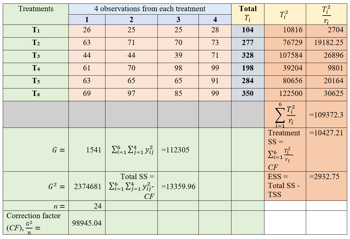
Figure 3.5: One-way ANOVA calculation
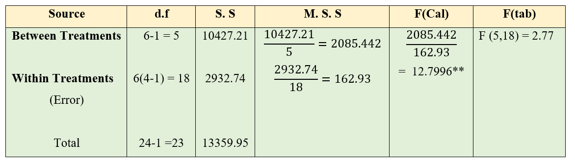
Figure 3.6: One-way table
Here you can see the calculated value is greater than table value of F. So the null hypothesis is rejected and we conclude that at least a pair of treatments are significantly different at 5% level of significance.
3.6.2 Two-way ANOVA
In one way ANOVA explained in the previous section, the treatments constitute different levels of a single factor which is controlled in the experiment. There are, however, many situations in which the response variable of interest may be affected by more than one factor. For example,
Milk yield of cow may be affected by differences in treatments i.e., feeds fed as well as differences in breed of the cows.
Moisture contents of butter prepared by churning cream may be affected with different levels of fat and churning speed etc.
Here two independent factors might have an effect on the response variable of interest. These two factors are considered to be the source of variation in the data in addition to experimental error. To compare means in such a situation we use two-way ANOVA.
In a two-way classification, the data are classified according to two different criteria or factors. The procedure for analysis of variance is somewhat different than the one followed earlier. One can also study interaction between the two factors, if interaction effect is included in two-way ANOVA model.
3.6.2.1 Two-way ANOVA model
\[Y_{\text{ij}} = \mu + \tau_{i} + \gamma_{j}+ e_{\text{ij}}\]
Where i = 1,2, …, t and j =1,2, …, r. \(Y_{\text{ij}}\) is the observed value of response under ith level of
factor A and jth level of factor B, \(\tau_{i}\) is the effect of ith factor,\(\gamma_{j}\) is the effect of jth factor . \(\mu\) is the general
effect which is common for all treatments. \(e_{\text{ij}}\) is the error
effects.\(e_{ij}\) \(\sim iid\ N(0,\sigma^{2})\)
3.6.2.2 Two-way classification
Consider an experiment with v levels of factor 1 with r levels of factor 2. Observations are recorded as shown below. We have considered the situation of only one observation per cell.
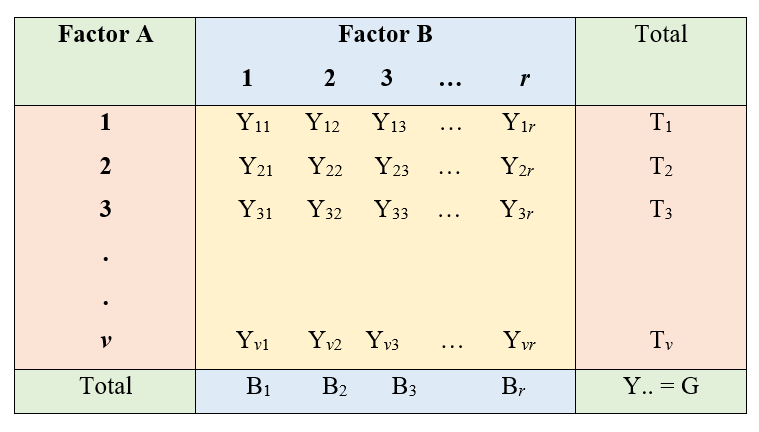
Figure 3.7: Two way classification of Data
3.6.2.3 Calculations for Two-way ANOVA
SSA = Take sum of squares of the totals of each level of factor A divide it by number of levels of factor B – Correction Factor
SSB = Take sum of squares of the totals of each level of factor B divide it by number of levels of factor A – Correction Factor.
Total SS = Take sum of squares of all observations – Correction Factor
Error SS = Total SS – SSA – SSB
Error Degrees of Freedom = Total D.F. – Factor A (D.F.) – Factor B (D.F.)
Error D.F.=
\(vr - 1 - \left( v - 1 \right) - \left( r - 1 \right) = vr - 1 - v + 1 - r + 1 = vr - v - r + 1 = (v - 1)(r - 1)\)
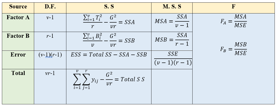
Figure 3.8: Two way ANOVA table
Here there are two F values one for factor A and one for Factor B. FA ~ F (v-1), (v-1)(r-1) and FB ~ F ~(r-1), (v-1)(r-1)
Here in Two-way ANOVA there are two null hypotheses one for factor A and other for factor B. For example for Factor A.
H0: \(\mu\)1 = \(\mu\)2 =\(\mu\)3 = …., = \(\mu\)v; where \(\mu\)i is the population mean of ith level of factor A. H1: atleast a pair of treatment means are not equal.
Factor B
H0: \(\beta\)1 = \(\beta\)2 =\(\beta\)3 = …., = \(\beta\)r; where \(\beta\)j is the population mean of jth level of factor B. H1: atleast a pair of treatment means are not equal.
Decisions on the null hypothesis is made by comparing corresponding F value to the table value as explained in section 6
3.6.2.4 Example of Two-way ANOVA
Four chemicals S1, S2, S3, and S4 were administered in 5 cow breeds (A, B, C, D, E). observations were taken during peak lactation period. Average yield over the period is taken. Is there any significant difference between chemicals? Is there any significant difference between milk yield of the breeds? Considering chemicals and breeds are independent.
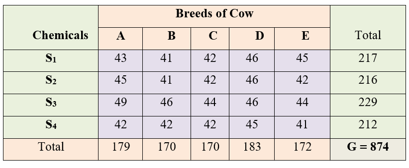
Figure 3.9: Two way classification of observations for chemicals and breeds
\(here\ n = 20,\ v = 5\ and\ r = 4\), factor A = cow breeds; factor B = chemicals, Grand total (G)=874
Correction Factor, \(CF = \frac{G^{2}}{n} = \frac{\left( 874 \right)^{2}}{20} = 38193.8\)
Total Sum of squares,
\(\text{TSS} = \text{sum of squares of all observations} - CF = \ \text{38288} - \text{CF} = \text{94.2}\)
Sum of Squares between Breeds (SSA)
\(= \sum_{i=1}^{v}\frac{T_{i}^{2}}{r} - \text{CF}\) \(= \frac{1}{4}\left\lbrack \left( \text{179} \right)^{2} + \text{...} + \left( \text{172} \right)^{2} \right\rbrack - \text{CF} = \text{34.7}\)
Sum of Squares between chemicals (SSB) \(= \sum_{j=1}^{r}\frac{B_{j}^{2}}{v} - \text{CF} = \frac{1}{5}\left\lbrack \left( \text{217} \right)^{2} + \text{...} + \left( \text{212} \right)^{2} \right\rbrack - \text{CF} = \text{32.2}\)
Sum of squares of Error
\(\text{SSE} = \text{TSS} - (\text{SST} + \text{SSB}) = \text{27.3}\)
Figure 3.10: ANOVA table for chemicals and breeds
For both chemicals and breeds there is significance difference at 5% level. Because both F values calculated are greater than table values.
3.7 Models under ANOVA
Analysis of variance is based on a linear statistical model. This linear model may be either
Fixed effects model
Random effects model
Mixed effects model
3.7.1 Fixed effects model
Fixed effects model is a statistical model in which the model parameters are fixed or non-random quantities. In using fixed effect model in agricultural experiments, we assume treatment effect are unknown constants
Fixed effects model can be explained using an example. Consider an experiment where experimenter wants to know whether three fields had any impact on the yield of a particular strain of wheat. Observations where taken from 12 plots from each fields (replication). The AOV (Analysis of Variance) model is
\(Y_{\text{ij}} = \mu + \tau_{i} + e_{\text{ij}}\); where \(e_{ij}\) \(\sim iid\ N(0,\sigma^{2})\)
Where i = 1,2, …, t and j =1,2, …, r. Here in our example t =3 and r =12. \(Y_{\text{ij}}\) is the observed value of ith field from jth plot, \(\tau_{i}\) is the effect of ith treatment, which is considered to be an unknown constant. \(\mu\) is the general effect which is common for all treatments. \(e_{\text{ij}}\) is the error effects, which are independently and normally distributed with mean 0 and constant variance σ2. In this model, field is a “fixed effect.” Along with \(\mu\), the fixed parameters \(\tau_{1}\),\(\tau_{2}\) and \(\tau_{3}\) are the quantities of interest. Using this model, experimenter can make decisions only on the treatment (field) tested.
3.7.2 Random effects model
A random effects model, also called as a variance components model, is a statistical model where the model parameters are random variables. Consider the example above in of wheat fields, if a random effect model is used then, fields are assumed to be randomly sampled from a population of fields in that area and the AOV (Analysis of Variance) model is
\(Y_{\text{ij}} = \mu + \tau_{i} + e_{\text{ij}}\);
\(e_{ij}\) \(\sim iid\ N(0,\sigma^{2})\) and \(\tau_{i}\sim N(0,\ \sigma_{\tau}^{2})\)
Where i = 1,2, …, t and j =1,2, …, r. Here \(\tau_{i}\) is considered as a random variable, \(\tau_{i}\sim N(0,\ \sigma_{\tau}^{2})\); and \(e_{ij}\sim N(0,\ \sigma^{2})\). In this model, field is a “random effect.” The statistical model describes the whole ensemble of possible repetitions of the experiment in the region from which the fields were selected. Experimenter could make generalisations on all the fields in that particular region based on his experiment. One important consequence of random effects is that the responses (\(Y_{\text{ij}}\)'s) are no longer independent. The random \(\tau_{i}\)'s induce correlations among the responses. The responses jointly have a multivariate normal distribution.
3.7.3 Mixed effects model
A mixed model, mixed-effects model or mixed error-component model is a statistical model containing both fixed effects and random effects.