5 Single factor experiments

Experiments in which only a single factor varies while all others are kept constant are called single-factor experiments. In such experiments, the treatments consist solely of the different levels of the single variable factor. All other factors are maintained uniformly in all other experimental units.

Example:

An experiment to find out the best nitrogen level for getting high yield, where 5 different nitrogen levels are tested. Here nitrogen levels are the treatments all other factors like irrigation, light, fertility gradient will be assumed to be homogenous in all experimental units (here plots are the experimental units).
An experiment to find out the best feed formulation for milk yield in cows from 4 feed formulas. Here feed formula is the only factor which varies with 4 levels. All other factors like breed of cow, age etc will be kept constant.

5.1 Completely Randomized Design (CRD)

Completely Randomized Design is the basic single factor design. In this design the treatments are assigned completely at random so that each experimental unit has the same chance of receiving any one treatment. CRD is only appropriate for experiments with homogeneous experimental units, such as laboratory and green house experiments, where environmental effects are relatively easy to control. For field experiments, where there is generally large variation among experimental plots, CRD is rarely used.

CRD provides a layout for conducting experiments, when experimental units are homogeneous. Only two basic principles of design, randomization 1.8.1 and replication1.8.2 are followed in CRD. Local control1.8.3 is not required as all the experimental units are homogeneous. Treatments can have unequal replications in CRD

5.1.1 Randomization procedure

Consider an experiment involving four treatments A, B, C, D in CRD. Each treatment is replicated 5 times. Randomization procedure is as explained below.

Determine the total number of experimental units (\(n\)) as the product of the number of treatments (\(t\)) and the number of replications (\(r\)); that is, \(n = r\ \times t\). For our example, \(n = 5 \times 4 = 20\)
Assign a unit number to each experimental units in any convenient manner; for example, consecutively from 1 to n. For our example, the unit numbers 1, ... , 20 are assigned to the 20 experimental units as shown in Figure 5.1
Assign the treatments to the experimental plots by using any randomization schemes. Here we explain a simple randomization scheme in section 5.1.1.1.

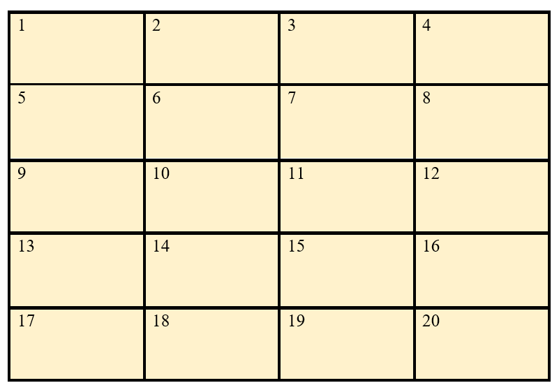
Figure 5.1: Numbered experimental units

5.1.1.1 Randomization by drawing lots

Prepare \(n\) identical pieces of paper and divide them into \(t\) groups, each group with \(r\) pieces of paper. Label each piece of paper of the same group with the same letter (or number) corresponding to a treatment. Uniformly fold each of the \(n\) labeled pieces of paper, mix them thoroughly, and place them in a container. For our example, there should be 20 pieces of paper, five each with treatments A, B, C, and D appearing on them.
Draw one piece of paper at a time, without replacement and with constant shaking of the container after each draw to mix its content. For our example, the label and the corresponding sequence in which each piece of paper is drawn. The sequence number can be considered as the experimental unit number to which the treatment is to be assigned.

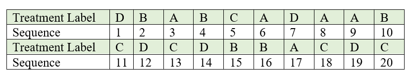
Figure 5.2: Sequence in which labelled lots are drawn

5.1.2 Layout of CRD

After allotting the treatment according to the randomization procedure explained in section 1.8.1. The final layout will look like in the figure 5.3.

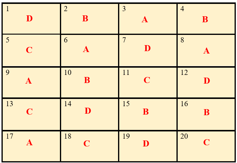
Figure 5.3: Layout of Completely Randomized Design

5.1.3 Statistical model for CRD

Consider a CRD with v treatments with r replications. Statistical model for CRD is same as that of one-way ANOVA (3.6.1.5).
\[Y_{\text{ij}} = \mu + \tau_{i} + e_{\text{ij}}\]
Where i = 1,2, …, v and j =1,2, …, r_i. \(Y_{\text{ij}}\) is the observed value of i^th treatment from j^th replication, \(\tau_{i}\) is the effect of i^th treatment. \(\mu\) is the general effect which is common for all treatments. \(e_{\text{ij}}\) is the error effects.\(e_{ij}\) \(\sim iid\ N(0,\sigma^{2})\)

5.1.4 Analysis of CRD

Analysis of CRD is same as that explained in section 3.6.1.5 of one-way ANOVA.

Note that unequal replication (i.e. each treatment can have different replication) is possible in CRD. So while calculating TSS, each treatment total square is divided by corresponding replication and then sum is taken. If the replication is same for all treatments, to calculate TSS take sum of all the squares of treatment total and then divide it by replication.

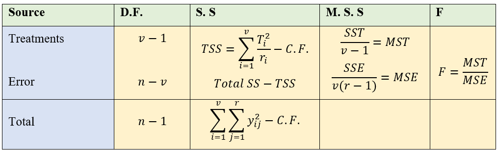
Figure 5.4: ANOVA table of CRD

5.1.4.1 Post hoc test (LSD)

If the null hypothesis is rejected in ANOVA; we proceed to post-hoc test explained in section . Fisher’s Least significant difference (LSD) test explained in section is the commonly employed test in agricultural experiments.
Arrange the treatment means in descending order. Critical difference (CD) is calculated for each treatment pair \(T_{i},\ T_{j}\) using the following formula.

\[C.D. = t_{\left( \frac{\alpha}{2},\ \ \ error\ df \right)}\sqrt{\text{MSE}\left( \frac{1}{r_{i}} + \frac{1}{r_{j}} \right)}\]

Here \(t_{\left( \frac{\alpha}{2},\ \ \ error\ df \right)}\) denotes the critical value of Student’s t for a two tailed test at α level of significance and error degrees of freedom. \(r_{i}\) and \(r_{j}\) are replications of \(T_{i},\ T_{j}\) respectively. If the difference of any two treatment means is greater than the critical difference, they are significantly different. If the difference of any two treatment means is less than \(\text{C.D}\). they are said to be on par. (i.e., there is no any statistically significant difference). Those treatments which are at par is given same symbols or letters, such that treatment means without any common letters or symbols are significantly different at corresponding level of significance (α).

5.1.5 Example

In order to find the yielding abilities of five varieties of sesame an experiment was conducted in the green house using a CRD with four pots per variety. The results are given in the following table below.

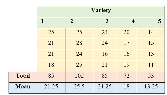
Figure 5.5: ANOVA table of CRD

5.1.5.1 Solution

Correction Factor:

\(= \frac{G^{2}}{n} = \frac{\left( 397 \right)^{2}}{20}\)=7880.45

Total Sum of squares:

\(= \left( 25^{2} + 21^{2} + .... + 11^{2} \right) - CF\)

\(= 8307 - CF = 426.55\)

Treatment Sum of Squares:

\(\frac{1}{4}(85^{2} + 102^{2} + ... + 53^{2}) - CF\)
\(= 8211.75 - CF = 331.30\)

Error Sum of Square:
\(426.55 - 331.30 = 95.25\)

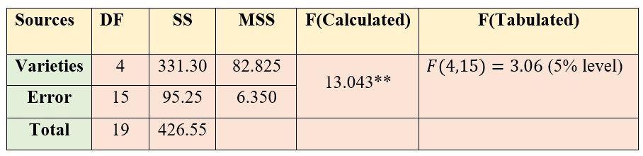
Figure 5.6: ANOVA table of CRD

Since the F value calculated is greater than table value of F, we can reject the null hypothesis and conclude that there is a significant difference between atleast a pair of treatments. So in order to find, which treatments are significantly different, we perform Fisher’s LSD test.

\[\text{CD} = t_{\frac{\alpha}{2}}\sqrt{\frac{\text{2xMSE}}{r}} = \text{2.131}\sqrt{\frac{2\left( \text{6.350} \right)}{4}} = (\text{2.131})(\text{1.7819}) = \text{3.797}\text{2}\]

\(t_{0.025\text{ at }15 \text{ edf}} = 2.131\) (Just look for the critical value of t for a two tailed test at α= 0.05 in the statistical table. (see section 6. It is shown as \(t_{\frac{\alpha}{2}}\) , since it is a two tailed test in the one side of the t-distribution curve the probability will be \(\frac{\alpha}{2}\), so that combined probability is α.)

Treatment means arranged in descending order. Those treatment pairs whose difference in means is greater than C.D. is labelled with a different letters.

Treatments	means	Grouping using alphabets
V2	25.5	a
V1	21.5	b
V3	21.5	b
V4	18	b
V5	13.5	c

In the above table we can see that difference between mean of V2 and V1 is 4 which is greater than C.D. value. So V2 and V1 are significantly different; different letters are assigned to each of them. Instead of letters one can also use symbols as shown below. Those treatments with same letters/symbols are not significantly different.

Treatments	means	Grouping using symbols
V2	25.5	@
V1	21.5	*
V3	21.5	*
V4	18	*
V5	13.5	&

So, in our example we can conclude that V2 is the best variety because, it is having the highest mean and is significantly different from others.

***************************************************************

Note: in some cases, more than one alphabets can appear against a treatment mean, see the hypothetical example below.

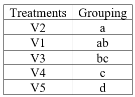
Figure 5.7: A hypothetical example of treatment grouping

If a lettering like this appears meaning is that those treatments having common alphabets are not significantly different. In the above table V2 and V1 is not significantly different as both of them are having common letter a. At the same time you can see V5 and V4 is significantly different as they don’t have any common letters.