2 Uniformity trials
Research worker would perform experiments in identical conditions to obtain valid results but even with the most uniform land that he can select, there will be still inherent variations in the soil. So, in order to maintain homogeneity, experimenter should have a good idea of the nature and extent of fertility variation in land. This can be obtained from the results of what are known as uniformity trials.
Uniformity trials can also be planned to determine suitable size and shape of the plot and the number of plots in a block. Uniformity trials enable us to have an idea about the fertility variation of the field.
2.1 How uniformity trial is performed
Uniformity trial was conducted to know the nature of the soil fertility gradient. Under uniformity trial, a particular variety of a crop will be sown on the entire experiment field and uniformly managed throughout the growing season without applying fertilizer. At the time of harvest a substantial border will be removed from all sides of the field. The remainder of the field will be divided into small plots which are termed as basic units. The size of the basic unit is decided by judgment, depending on the crop. Smaller the basic unit more accurate study on heterogeneity is possible. The produce from the basic unit will be harvested and recorded separately for each basic unit. The yield differences between the basic units are taken as the measure of soil heterogeneity of the study area.
Several types of analysis are available to evaluate pattern of soil heterogeneity based on uniformity trial data. We will discuss some of the procedures in detail.
2.2 Fertility Contour Map
An approach to describe the heterogeneity of land is to construct the fertility contour map. It is simple but informative presentation of soil heterogeneity. This is constructed by taking the moving averages of yields of unit plots and demarcating the regions of same fertility by considering those areas, which have yield of same magnitude. Taking moving average reduce the large random variation expected on small plots.
2.3 Serial Correlation
Serial correlation procedure is generally used to test the randomness of a data set. However, it is also useful in the characterization of the trend in soil fertility using uniformity trial data. Horizontal and vertical serial correlations were calculated. These correlations give idea on whether fertility gradient was more pronounced horizontally or vertically. A low serial correlation indicates that fertile areas occur in spots and a high value indicates there is a gradient.
\[r_{s} = \frac{\sum_{i = 1}^{n}{X_{i}X_{i + 1} - \frac{\left( \sum_{i = 1}^{n}X_{i} \right)^{2}}{n}}}{\sum_{i = 1}^{n}{X_{i}}^{2} - \frac{\left( \sum_{i = 1}^{n}X_{i} \right)^{2}}{n}}\]
where \(X_{i}\) is the value of ith basic unit and \(n\) is the number of basic units.
2.4 Mean square between strips
This method is simpler to compute and it has the objective same as the serial correlation. Units are first combined as horizontal and vertical strips. Variability between strips were measured in each direction by mean square between strips. The relative size of two mean squares indicates whether fertility gradient was more pronounced horizontally or vertically.
\[\text{Sum of square}\left( \text{Vertical} \right)\frac{\sum_{i = 1}^{c}V_{i}^{2}}{r} - \frac{G^{2}}{n}\ \]
\[\text{Sum of square}\left( \text{Horizontal} \right)\frac{\sum_{i = 1}^{c}H_{i}^{2}}{c} - \frac{G^{2}}{n}\ \]
\[\text{mean square}\left( \text{Vertical} \right) = \frac{\text{Sum of square}\left( \text{vertical} \right)}{c - 1}\]
\[\text{mean square}\left( \text{Horizontal} \right) = \frac{\text{Sum of square}\left( \text{Horizontal} \right)}{r - 1}\]
where \(V_{i},H_{i}\) are sum total of basic units in vertical and horizontal strips respectively; \(r\) is the number of rows and \(c\) is the number of columns. \(n\) is the total number of basic units; \(n = r \times c\). \(G\) is the total of all the basic units.
2.5 Fairfield Smith’s Variance Law
Smith (1938) gave a empirical relations between variance and plot size. He developed an empirical model representing the relationship between plot size and variance of mean per plot. This model is given by the equation
\[V_{x} = \frac{V_{1}}{x^{b}}\]
\[\log V_{x} = \ \log V_{1} - b\log x\]
where \(x\) is number of basic units in a plot, \(V_{x}\) is the variance of mean per plot of \(x\) units, \(V_{1}\) is the variance of mean per plot of one unit, and \(b\) is the regression coefficient. The values of \(b\) is determined by the principle of least squares. \(b\) is called Smith’s index of soil heterogeneity. The index gives a single value as quantitative measure of heterogeneity in the area.
2.5.1 Smith’s index of soil heterogeneity
Step-1 Combine the basic units to simulate plots of different sizes and shapes. Use only combinations that fit exactly into the whole area,i.e. the product of simulated plots and the number of basic units per plot must equal to the total number of basic units.
Step-2 For each of the simulated plots constructed in Step-1, compute the yield total T as the sum of basic units to construct that plot and compute between plot variance \(V_{(x)}\)
\[V_{(x)} = \sum_{i = 1}^{w}\frac{{T_{i}}^{2}}{x} - \frac{\left( G \right)^{2}}{\text{rc}}\]
where \(w = \frac{\text{rc}}{x}\ \)is the total number of simulated plots of size\(\text{\ x}\) basic units. \(r\) is the number of rows and \(c\) is the number of columns. \(G\) is the total of all the basic units.
Step-3 For each plot size and shape, compute the variance per unit area
\[V_{x} = \frac{V_{(x)}}{rc - 1}\]
Step-4 For each plot size having more than one shape, test the homogeneity of between-plot variances \(\mathbf{V}_{\left( \mathbf{x} \right)}\)to determine the significance of plot orientation (plot-shape) effect, by using the F test or the chi-square test. If found homogeneous, the average of \(\mathbf{V}_{\mathbf{(x)}}\) values over all plot shapes of a given size is computed, otherwise \(\mathbf{V}_{\mathbf{(x)}}\)of each plot shapes of a given size is used separately for further calculation.
For example, there are two plot shapes for size 2m2 i.e. 2 × 1m and 1 × 2m. For both these plot \(\mathbf{V}_{\mathbf{(x)}}\)is calculated. Homogeneity is tested using F test. If it is non-significant the average of \(\mathbf{V}_{\mathbf{(x)}}\) values over the plot shapes 2 × 1m and 1 × 2m will be calculated.
Step-5 Using the values of the variance per unit area \(\mathbf{V}_{\mathbf{x}}\) computed in steps 3 and 4, estimate the regression coefficient between \(\mathbf{V}_{\mathbf{x}}\) and plot size \(\mathbf{x}\)
Using Fairfield Smith’s Variance Law, which can be written by taking logarithm to the base e as:
\[\log V_{x} - \log V_{1} = \ - b\log x\]
consider
\[{Y = \log}V_{x} - \log V_{1}\]
then equation \(\log V_{x} - \log V_{1} = \ - b\log x\) can be written in the form
\(\mathbf{Y = \ cX}\) where \(\mathbf{c = \ - b;\ X =}\mathbf{\log}\mathbf{x}\)
\(\mathbf{b}\) is estimated by fitting regression between \(\mathbf{Y}\) and \(\mathbf{X}\).
Step-6 Obtain the adjusted \(\mathbf{b}\) from the computed \(\mathbf{b}\) value using the range \(\frac{\mathbf{x}_{\mathbf{1}}}{\mathbf{n}}\),
where\(\mathbf{\ }\mathbf{x}_{\mathbf{1}}\), is the size of basic unit and
\(\mathbf{n}\) is the whole area size. Column 2 and 3 in the table 2.1 is the range of \(\frac{\mathbf{x}_{\mathbf{1}}}{\mathbf{n}}\). once you get the computed \(b\) and value of \(\frac{\mathbf{x}_{\mathbf{1}}}{\mathbf{n}}\). You can calculate the corresponding adjusted \(b\) using the table 2.1. using interpolation as follows.
Find L1 and L2 such that, calculated b lies between them;
L1 ≤ bcal ≤ L2, where L1 and L2 are the values in
computed b column in table 2.1. Let y1 , y2 be the value
corresponding to L1 and L2 under the range of \(\frac{\mathbf{x}_{\mathbf{1}}}{\mathbf{n}}\) in the table 2.1. Then using the formula
Adjusted b value = \(y_{1} + (b_{\text{cal}} - L_{1})\frac{\left( y_{2} - y_{1} \right)}{\left( L_{2} - L_{1} \right)}\)
| Computed b | Range 0.001 to 0.01 | Range 0.01 to 0.1 |
| 1 | 1 | 1 |
| 0.8 | 0.804 | 0.822 |
| 0.7 | 0.71 | 0.738 |
| 0.6 | 0.617 | 0.656 |
| 0.5 | 0.528 | 0.578 |
| 0.4 | 0.443 | 0.504 |
| 0.35 | 0.403 | 0.469 |
| 0.3 | 0.364 | 0.434 |
| 0.25 | 0.326 | 0.402 |
| 0.2 | 0.291 | 0.371 |
| 0.1 | 0.257 | 0.343 |
| 0.15 | 0.226 | 0.312 |
A relatively low value of calculated adjusted Smith's index of soil heterogeneity (\(\mathbf{b}\)) indicates a relatively high degree of correlation among adjacent plots in the study area, which indicates the change in the level of soil fertility tends to be gradual rather than in patches. Even though \(\mathbf{b}\) is a regression coefficient its value lies between 0 and 1.
2.6 Maximum Curvature Method
This method is used to find optimal plot size for the experiment. In this method basic units of uniformity trials are combined to form new units. The new units are formed by combining columns, rows or both. Combination of columns and rows be done in such a way that no columns or rows is left out. For each set of units, the coefficient of variation (CV) is computed. A curve is plotted by taking the plot size (in terms of basic units) on X-axis and the CV values on the Y-axis of graph sheet. The point at which the curve takes a turn, i.e., the point of maximum curvature is located by inspection. The value corresponding to the point of maximum curvature will be optimum plot size.
2.7 Uniformity trial explained
Let us discuss in detail the procedures explained above using an example. Consider a rice crop field of 12m × 17m uniformly managed throughout the growing season without applying fertilizer. At the time of harvest a border of 1m is removed from all sides of the field. The resultant effective area is now 10m × 15m, entire field is divided in basic units of size 1m × 1m, and yield (in gms) were noted from each basic unit. There are 150 basic units.
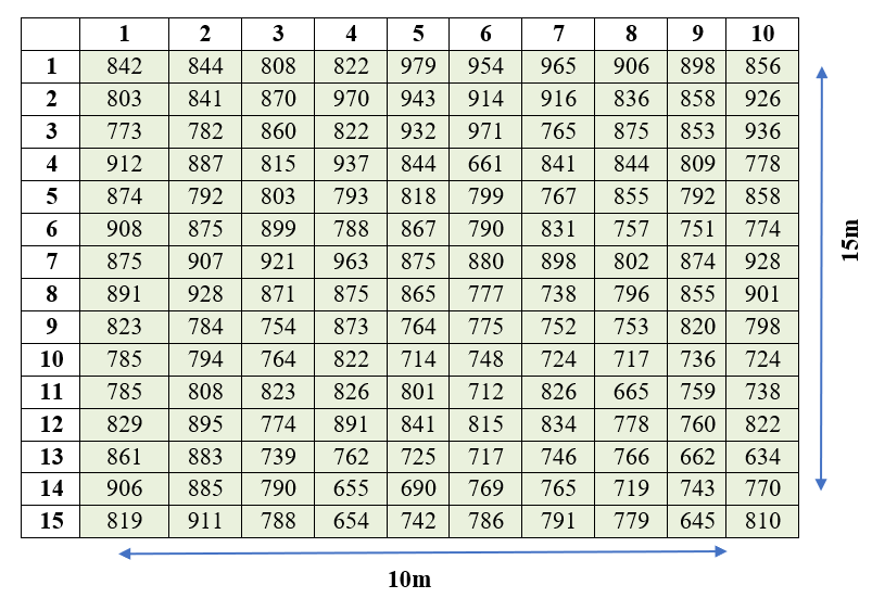
Figure 2.1: Yield observed from the plots of 1x1m size
Note: here r=15;c=10 and total number of basic units n=r×c=150
2.7.1 Fertility contour map
Also known as soil productivity contour map. construction fertility contour map is explained using above example.
Step 1: Calculate moving averages of 3m×3m basic units. i.e including three basic units in rows and 3 basic units in columns.
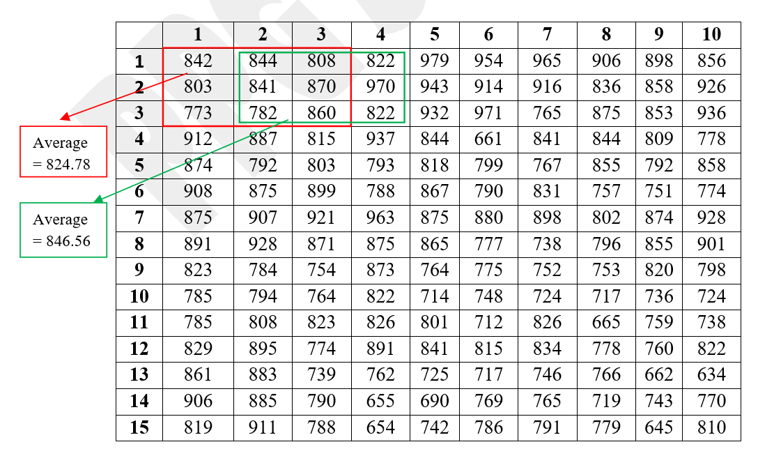
Figure 2.2: Calculation of moving averages of 3m×3m basic units
Step 2: Moving averages where labeled as shown below. After calculation of moving averages now there are 8 values in a row and 13 values in a column. Now the dimension of each plot in the figure below can be considered as 1.25m × 1.154m (10/8 = 1.25 and 15/13 = 1.514)
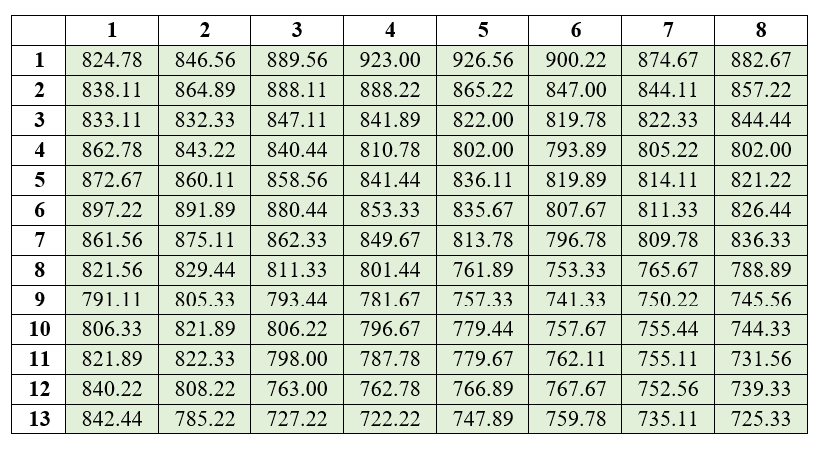
Figure 2.3: Moving averages recorded for all 3m×3m basic units
Step 3: Similar areas where given same colours to get a fertility contour map.
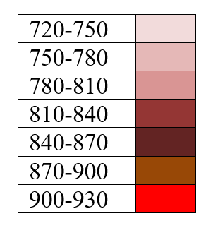
Figure 2.4: Colouring scheme based on range of moving averages. This can be decided by the experimenter
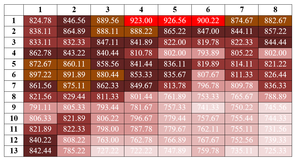
Figure 2.5: Coloured plot labelled with moving averages
Final fertility contour map is obtained as shown in figure 2.7. Now you can get an idea of fertility gradient of the field and plan how to create blocks in the field.
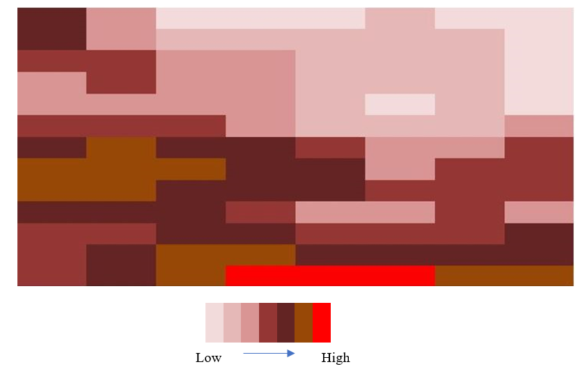
Figure 2.6: Final fertility contour map
Fertility contour map gives only a vague idea of fertilizer gradient. Other procedures may give a better idea.
2.7.2 Serial Correlation
Pair wise calculation of vertical values from the experiment observations shown in figure 2.1
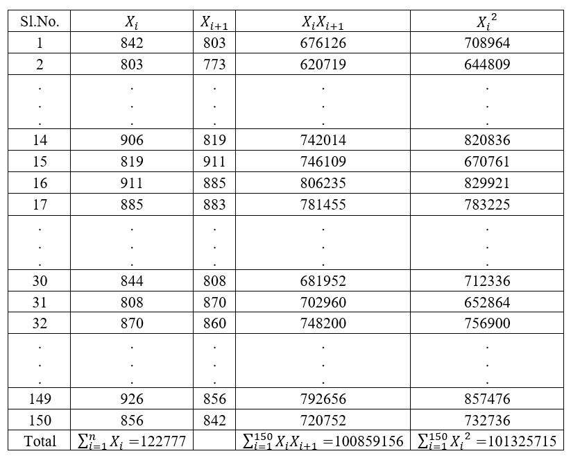
Figure 2.7: Pair wise calculation of vertical values
Using
\(r_{s} = \frac{\sum_{i = 1}^{n}{X_{i}X_{i + 1} - \frac{\left( \sum_{i = 1}^{n}X_{i} \right)^{2}}{n}}}{\sum_{i = 1}^{n}{X_{i}}^{2} - \frac{\left( \sum_{i = 1}^{n}X_{i} \right)^{2}}{n}}\)
Vertical \(r_{s} = \frac{100859156 - \frac{\left( 122777 \right)^{2}}{150}}{101325715 - \frac{\left( 122777 \right)^{2}}{150}}\ \)= 0.438627
Pair wise calculation of Horizontal values shown in figure 2.1
Figure 2.8: Pair wise calculation of horizontal values
Using
\[r_{s} = \frac{\sum_{i = 1}^{n}{X_{i}X_{i + 1} - \frac{\left( \sum_{i = 1}^{n}X_{i} \right)^{2}}{n}}}{\sum_{i = 1}^{n}{X_{i}}^{2} - \frac{\left( \sum_{i = 1}^{n}X_{i} \right)^{2}}{n}}\]
Horizontal \(r_{s} = \frac{100946042 - \frac{\left( 122777 \right)^{2}}{150}}{101325715 - \frac{\left( 122777 \right)^{2}}{150}}\ \)= 0.54317
Both coefficients are low which indicates the presence of fertile areas in spots. However, the horizontal serial correlation coefficient was little high than vertical implying that some fertility gradient in horizontal direction than vertical. The relative magnitude of the two serial correlations should not, however, be used to indicate the relative degree of the gradients in the two directions.
2.7.3 Mean square between strips
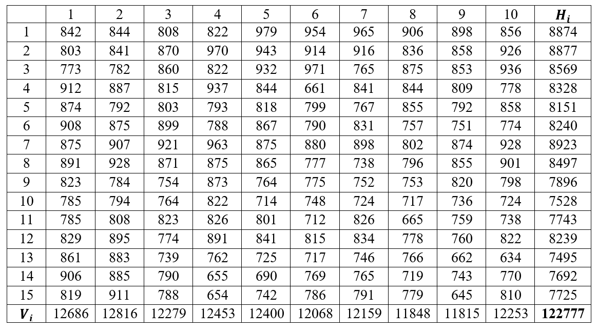
Figure 2.9: Mean square between strips from uniformity trial data
\(G =\) 122777, \(n =\) 150
\(\text{Sum}\ \text{of}\ \text{square}\left( \text{vertical} \right)\frac{\sum_{i = 1}^{c}V_{i}^{2}}{r} - \frac{G^{2}}{n} = \frac{12686^{2} + 12816^{2} + \ldots 12253^{2}}{15} - \frac{122777^{2}}{150}\) = 63971.47
\(\text{Sum}\ \text{of}\ \text{square}\left( \text{Horizontal} \right)\frac{\sum_{i = 1}^{c}H_{i}^{2}}{c} - \frac{G^{2}}{n} = \frac{8874^{2} + 8877^{2} + \ldots 7692^{2}}{10} - \frac{7725^{2}}{150}\ \)= 341185.7733
\(\text{mean}\ \text{square}\left( \text{vertical} \right) = \frac{63971.47}{9}\ \)= 7107.941481
\(\text{mean}\ \text{square}\left( \text{Horizontal} \right) = \frac{341185.773}{14}\ \)= 24370.41238
Results show that the horizontal-strip MS is almost 3 times higher than the vertical-strip MS, indicating that the trend of soil fertility was more pronounced along the length than along width of the field.
2.7.4 Smith’s index of soil heterogeneity
Optimal plot size can be identified using this method. From the possible plot sizes optimum plot size can be found out using method explained in section 2.5.1. Table below shows 9 different plot sizes created from uniformity trial data in figure 2.1.
| Sl. No. | Size of plot (x) |
Width | Length | No: of plots (\(w\)) |
|---|---|---|---|---|
| 1 | 1 | 1 | 1 | 150 |
| 2 | 2 | 2 | 1 | 75 |
| 3 | 3 | 1 | 3 | 50 |
| 4 | 5 | 1 | 5 | 30 |
| 5 | 5 | 5 | 1 | 30 |
| 6 | 6 | 2 | 3 | 25 |
| 7 | 10 | 2 | 5 | 15 |
| 8 | 15 | 5 | 3 | 10 |
| 9 | 25 | 5 | 5 | 6 |
It is recommended that the reader should first read section 2.5.1 and then read this example. Here, I will illustrate how variance per unit area for a plot of size 25m2 (denoted as V25) is calculated. The width and length of the plot is 5m × 5m. The entire plot area in figure 2.1 is divided in to six plots of size 25m2 as shown below.
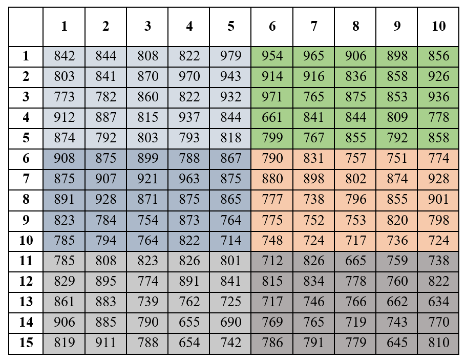
Figure 2.10: Uniformity trail plot in figure 2.1 is divided in to six plots
Now consider the equation for between plot variance \(V_{(x)} = \sum_{i = 1}^{w}\frac{{T_{i}}^{2}}{x} - \frac{\left( G \right)^{2}}{\text{rc}}\). where \(w = \frac{\text{rc}}{x}\ \)is the total number of simulated plots of size\(\text{\ x}\) basic units. \(r\) is the number of rows and \(c\) is the number of columns. \(G\) is the total of all the basic units.
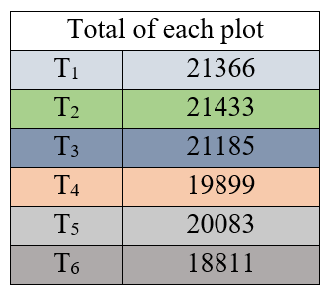
Figure 2.11: Totals of each of six plots
\(V_{(25)} = \frac{21366^{2} + 21433^{2}\ldots + 18811^{2}}{25} - \frac{\left( 122777 \right)^{2}}{150} = \ \)218767.7133
Variance per unit area is given by \(V_{x} = \frac{V_{(x)}}{rc - 1}\)
\(V_{25} = \frac{218767.7133}{149}\ = \ \)1468.24
Coefficient of variation is calculated as \(\frac{\text{Standard\ deviation}}{\text{mean}} \times 100\), here in this example of plot size 25. Standard deviation= \(\sqrt{1468.24}\) = 38.31762. Mean of entire data set = 818.5133. Therefore C.V = \(\frac{38.31762}{818.5133} = 0.047\). Similarly, it can be calculated for all the plot sizes. Vx and C.V for all other plot sizes are summarized below.
| Sl. No. | Size of plot (x) |
Width | Length | No: of plots (\(w\)) |
Vx | C.V |
|---|---|---|---|---|---|---|
| 1 | 1 | 1 | 1 | 150 | 5577.88 | 9.1 |
| 2 | 2 | 2 | 1 | 75 | 4427.18 | 8.1 |
| 3 | 3 | 1 | 3 | 50 | 3733.36 | 7.5 |
| 4 | 5 | 1 | 5 | 30 | 2213.82 | 5.7 |
| 5 | 5 | 5 | 1 | 30 | 3066.42 | 6.8 |
| 6 | 6 | 2 | 3 | 25 | 3316.61 | 7 |
| 7 | 10 | 2 | 5 | 15 | 2003.03 | 5.5 |
| 8 | 15 | 5 | 3 | 10 | 2268.41 | 5.8 |
| 9 | 25 | 5 | 5 | 6 | 1468.24 | 4.7 |
For each plot size having more than one shape (here plot size 5 have more than one shape), test the homogeneity of between-plot variances V(x), to determine the significance of plot orientation (plot-shape) effect, by using the F test or the chi-square test. For each plot size whose plot-shape effect is non-significant, compute the average of Vx, values over all plot shapes and proceed with estimation of Smith's index of soil heterogeneity.
V(x) calculated for both plot sizes
| Plot shapes | V(x) |
|---|---|
| 1×5 | 456895.9 |
| 5×1 | 329859.5 |
Degrees of freedom for F test are \((w_{1} - 1,\ w_{2} - 1)\), where \(w_{1}\) and \(w_{2}\) are number of plots of particular shapes each. Here, degrees of freedom = (30-1, 30-1)=(29,29). F is calculated as the ratio of V(x) of both plot shapes. Fcal= \(\frac{456895.9}{329859.5}\) =1.38. Calculated value of F (Fcal) is compared with table value of F. Table value of F at (29,29) degrees of freedom, Ftable= 1.860. Since Fcal < Ftable; Calculated F is non-significant, so take average of Vx of both plot shapes and proceed. In our example we proceeded without taking the average. I included this example of F test for a better understanding of the theory written.
Now Smith's index of soil heterogeneity is estimated as follows
Size of plot (x) |
Vx | log(Vx) | Y = log(Vx) -log(V1) | X = log(x) |
|---|---|---|---|---|
| 1 | 5577.88 | 8.62656 | 0 | 0 |
| 2 | 4427.18 | 8.39552 | -0.231045 | 0.6931472 |
| 3 | 3733.36 | 8.22506 | -0.401499 | 1.0986123 |
| 5 | 2213.82 | 7.70248 | -0.924087 | 1.6094379 |
| 5 | 3066.42 | 8.02826 | -0.598299 | 1.6094379 |
| 6 | 3316.61 | 8.1067 | -0.519865 | 1.7917595 |
| 10 | 2003.03 | 7.60242 | -1.024146 | 2.3025851 |
| 15 | 2268.41 | 7.72683 | -0.899731 | 2.7080502 |
| 25 | 1468.24 | 7.29182 | -1.334744 | 3.2188758 |
| V1 = 5577.88; log(V1) = 8.62656 |
Fit a linear regression Y = cX, estimate the value of c; c= -b
Estimated value of c is -0.3952. Therefore, calculated value of b = 0.3952. In our case \(\text{}\frac{x_{1}}{n} = \frac{1}{150} = 0.0067\). Now we need to find the adjusted value as explained in step-6 in section 2.5.1 using the table below.The value of \(\frac{x_{1}}{n} = \frac{1}{150} = 0.0067\) is between 0.001 and 0.01.
Here \(b_{\text{cal}}\)= 0.3952
\(y_{1}\) = 0.443
\(y_{2}\) = 0.528
\(L_{1}\)= 0.40
\(L_{2}\) = 0.50
Adjusted b value = \(0.443 + (0.3952 - 0.40)\frac{\left( 0.528 - 0.443 \right)}{\left( 0.50 - 0.40 \right)}\) = 0.43892.
Computed b |
0.001 to 0.01 | 0.01 to 0.1 |
|---|---|---|
| 1.00 | 1.000 | 1.000 |
| 0.80 | 0.804 | 0.822 |
| 0.70 | 0.710 | 0.738 |
| 0.60 | 0.617 | 0.656 |
| 0.50 | 0.528 | 0.578 |
| 0.40 | 0.443 | 0.504 |
| 0.35 | 0.403 | 0.469 |
| 0.30 | 0.364 | 0.434 |
| 0.25 | 0.326 | 0.402 |
| 0.20 | 0.291 | 0.371 |
| 0.10 | 0.257 | 0.343 |
| 0.15 | 0.226 | 0.312 |
If \(b\) value is low it indicates a relatively high degree of correlation among adjacent plots in the study area indicating a gradual change in soil fertility. But here \(b\) is 0.43892, which is moderate, so there is no indication of gradient but slight indication of patches.
2.7.5 Maximum Curvature Method
This method (see section 2.6) is used to find optimum plot size. A curve is plotted by taking the plot size (in terms of basic units) on X-axis and the CV values on the Y-axis.
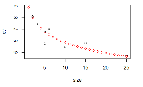
Figure 2.12: Relationship between CV and plot size
Figure 2.12indicates that as the plot size increases, coefficients of variation decreases and this decrease is maximum with the square shape plot of 5m×5m. As we took a small data set for illustrative purpose, it is clearly seen that 5m×5m plot has the lowest CV value and also lowest variance per basic unit area.
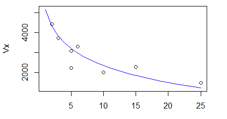
Figure 2.13: Relationship between variance per basic unit area and plot size
Figure 2.13 shows the relationship between variance per basic unit area Vx and plot size (x)