3 Measures of Central Tendency - I
In the previous chapter, you have learnt how data can be summarised in the form of tables and presented in the form of graphs so that important features can be illustrated easily and more effectively. In this Lecture, we consider statistical measures which can be used to describe the characteristics of a set of data.
We are interested in a single value that serves as a representative value of the overall data. A measure of central tendency is a summary statistic that represents the centre point or typical value of a dataset.
There are five averages. Among them mean, median and mode are called simple averages and the other two averages geometric mean and harmonic mean are called special averages. These measures reflect numerical values in the centre of a set of data and are therefore called measures of central tendency.
Requisites of a Good Measure of Central Tendency:
It should be rigidly defined.
It should be simple to understand & easy to calculate
It should be based upon all values of given data
It should be capable of further mathematical treatment.
It should have sampling stability.
It should be not be unduly affected by extreme values
The main objectives of Measure of Central Tendency:
To condense data in a single value.
To facilitate comparisons between data.
3.1 Arithmetic Mean
This is what people usually intend when they say “average”. Arithmetic mean or simply the mean of a variable is defined as the sum of the observations divided by the number of observations. Mean of set of numbers \(x_{1\ },x_{2},\ldots,x_{n}\) is denoted as \(\overline{x}\). It is given by the formula
\[\overline{x} = \frac{x_{1} + x_{2} + \ldots + x_{n}}{n}\]
\[= \frac{1}{n}\sum_{i = 1}^{n}x_{i}\]
Example 3.1 Find the mean of the numbers 2, 4, 7, 8, 11, 12
\[\overline{x} = \frac{2 + 4 + 7 + 8 + 11 + 12}{6} = \frac{44}{6} = 7.33\]
3.1.1 The mean of a frequency distribution
3.1.1.1 Direct method
If the numbers \(x_{1\ },x_{2},\ldots,x_{n}\) occur with frequencies \(f_{1\ },f_{2},\ldots,f_{n}\) respectively then
\[\overline{x} = \frac{x_{1}f_{1} + x_{2}f_{2\ \ } + \ldots + x_{n}f_{n}}{f_{1} + f_{2} + \ldots f_{n}}\]
\[= \frac{\sum_{i = 1}^{n}{f_{i}x_{i}}}{\sum_{i = 1}^{n}f_{i}}\]
Example 3.2 Table below shows the plant height of 50 plants. Find the mean plant height.
| Plant height(cm) | 159 | 160 | 161 | 162 | 163 |
|---|---|---|---|---|---|
| Frequency | 3 | 9 | 23 | 11 | 4 |
Solution 3.2
The calculation can be arranged as shown
| Plant height(x) | Frequency(f) | fx |
|---|---|---|
| 159 | 3 | 477 |
| 160 | 9 | 1440 |
| 161 | 23 | 3703 |
| 162 | 11 | 1782 |
| 163 | 4 | 652 |
| \(\sum_{i = 1}^{n}f_{i}\)= 50 | \(\sum_{i = 1}^{n}{f_{i}x_{i}}\)= 8054 |
\(\overline{x} = \frac{\sum_{i = 1}^{n}{f_{i}x_{i}}}{\sum_{i = 1}^{n}f_{i}} = \frac{8054}{50}\)= 161.08 cm
3.1.1.2 Assumed mean method (Indirect method)
The amount of computation involved above can be reduced by using the following formula:
\[\overline{x} = A + \frac{\sum_{i = 1}^{n}{f_{i}d_{i}}}{\sum_{i = 1}^{n}f_{i}}\]
Where \(A\) is the assumed mean, which can be any value in x. \(d_{i} = x_{i} - A\), \(f_{i}\) is the frequency of \(x_{i}\)
Consider the Example 3.2
let \(A\) = 161; it can be any number in x
| Plant height(x) | Frequency(f) | \[\mathbf{d}_{\mathbf{i}}\mathbf{=}\mathbf{x}_{\mathbf{i}}\mathbf{-}\mathbf{161}\] | \(\mathbf{f}_{\mathbf{i}}\mathbf{d}_{\mathbf{i}}\) |
|---|---|---|---|
| 159 | 3 | -2 | -6 |
| 160 | 9 | -1 | -9 |
| 161 | 23 | 0 | 0 |
| 162 | 11 | 1 | 11 |
| 163 | 4 | 2 | 8 |
| \(\sum_{i = 1}^{n}f_{i}= 50\) | \(\sum_{i = 1}^{n}{f_{i}d_{i}}\)= 4 |
\(\overline{x} = 161 + \frac{4}{50}\) = 161.08 cm
The mean plant height is 161.08 cm
3.1.2 Mean of Grouped Data
3.1.2.1 Direct method
The mean for grouped data is obtained from the following formula:
\[\overline{x} = \frac{\sum_{i = 1}^{k}{f_{i}x_{i}}}{n}\]
Where \(x_{i}\) = the mid-point of ith class (ith class mark); \(f_{i}\)= the frequency of ith class; \(n\) = the sum of the frequencies or total frequencies in a sample. Note that i =1,2..., k, i.e. there are k classes.
Example 3.3 Shows the distribution of the marks scored by 60 students in a Maths examination. Find the mean mark.
| Mark (%) | 60-65 | 65-70 | 70-75 | 75-80 | 80-85 |
|---|---|---|---|---|---|
| Number of students | 2 | 15 | 25 | 14 | 4 |
Solution 3.3
The solution can be arranged as shown
| Marks | Class mark(\(\mathbf{x}_{\mathbf{i}}\)) | Frequency(\(\mathbf{f}_{\mathbf{i}}\)) | \[\mathbf{f}_{\mathbf{i}}\mathbf{x}_{\mathbf{i}}\] |
|---|---|---|---|
| 60-65 | 62.5 | 2 | 125 |
| 65-70 | 67.5 | 15 | 1012.5 |
| 70-75 | 72.5 | 25 | 1812.5 |
| 75-80 | 77.5 | 14 | 1085 |
| 80-85 | 82.5 | 4 | 330 |
| \(\sum_{i = 1}^{n}f_{i}\)= 60 | \(\sum_{i = 1}^{n}{f_{i}x_{i}}\)= 4365 |
\(\overline{x} = \frac{\sum_{i = 1}^{n}{f_{i}x_{i}}}{\sum_{i = 1}^{n}f_{i}} = \frac{4365}{60}\)= 72.75
The mean mark is 72.75%
3.1.2.2 Coding method (Indirect method)
If all the class intervals of a grouped frequency distribution have equal size \(C\) (class width); then the following formula can be used instead of direct method above. This formula makes calculations easier.
\[\overline{x} = A + C\frac{\sum_{i = 1}^{n}{f_{i}u_{i}}}{\sum_{i = 1}^{n}f_{i}}\]
Where \(A\) is the class mark with the highest frequency, \(u_{i} = \frac{x_{i} - A}{C}\), \(f_{i}\) is the frequency of \(x_{i}\), C is the class width.
This is called the “coding” method for computing the mean. It is a very short method and should always be used for finding the mean of a grouped frequency distribution with equal class widths.
Consider the Example 3.3 see Table:3.2
\(A\)=72.5, class mark with highest frequency; \(C\) =5
| Marks | Class mark(\(\mathbf{x}_{\mathbf{i}}\)) | Frequency(\(\mathbf{f}_{\mathbf{i}}\)) | \[\mathbf{u}_{\mathbf{i}}\mathbf{=}\frac{\mathbf{x}_{\mathbf{i}}\mathbf{- 72.5}}{\mathbf{5}}\] | \[\mathbf{f}_{\mathbf{i}}\mathbf{u}_{\mathbf{i}}\] |
|---|---|---|---|---|
| 60-65 | 62.5 | 2 | -2 | -4 |
| 65-70 | 67.5 | 15 | -1 | -15 |
| 70-75 | 72.5 | 25 | 0 | 0 |
| 75-80 | 77.5 | 14 | 1 | 14 |
| 80-85 | 82.5 | 4 | 2 | 8 |
| \(\sum_{i = 1}^{k}f_{i}\)= 60 | \(\sum_{i = 1}^{k}{f_{i}u_{i}}\)=3 |
\(\overline{x} = 72.5 + 5 \times \left( \frac{3}{60} \right)\)= 72.75
The mean mark is 72.75%
3.1.3 Merits and demerits of Arithmetic mean
Merits
It is rigidly defined.
It is easy to understand and easy to calculate.
If the number of items is sufficiently large, it is more accurate and more reliable.
It is a calculated value and is not based on its position in the series.
It is possible to calculate even if some of the details of the data are lacking.
Of all averages, it is affected least by fluctuations of sampling.
It provides a good basis for comparison.
Demerits
It cannot be obtained by inspection nor located through a frequency graph.
It cannot be in the study of qualitative phenomena not capable of numerical measurement i.e. Intelligence, beauty, honesty etc.
It can ignore any single item only at the risk of losing its accuracy.
It is affected very much by extreme values.
It cannot be calculated for open-end classes.
It may lead to fallacious conclusions, if the details of the data from which it is computed are not given.
3.2 The Median
The median of a set of data is defined as the middle value when the data is arranged in order of magnitude. If there are no ties, half of the observations will be smaller than the median, and half of the observations will be larger than the median. The median can be the middle most item that divides the group into two equal parts, one part comprising all values greater, and the other, all values less than that item. It is a positional measure.
3.2.1 Median of ungrouped or raw data
Arrange the given n observations \(x_{1\ },x_{2},\ldots,x_{n}\) in ascending order. If the number of values is odd, median is the middle value. If the number of values is even, median is the mean of middle two values.
Arrange data in ascending then use the following formula
When n is odd, Median = Md =\(\left( \frac{n + 1}{2} \right)^{\text{th}}\)value
When n is even, Median = Md =\({\text{Average of}\left( \frac{n}{2} \right)^{th}\text{and }\left( \frac{n}{2} + 1 \right)}^{\text{th}}\)value
Example 3.4 Find the median of each of the following sets of numbers.
\(a)\) 12, 15, 22, 17, 20, 26, 22, 26, 12
\(b)\) 4, 7, 9, 10, 5, 1, 3, 4, 12, 10
Solution 3.4
\(a)\) Arranging the data in an increasing order of magnitude, we obtain 12, 12, 15, 17, 20, 22, 22, 26, 26. Here, N = 9 is odd, and so, median =\(\left( \frac{9 + 1}{2} \right)^{\text{th}}\)= 5th ordered observation = 20.
Note: If a number is repeated, we still count it the number of times it appears when we calculate the median.
\(b)\) Arranging the data in an increasing order of magnitude, we obtain 1, 3, 4, 4, 5, 7, 9, 10, 10, 12. Here, N = 10 is an even number and so median = \(\frac{1}{2}\){5th ordered observation + 6th ordered observation} = \(\frac{1}{2}\left( 5 + 7 \right) = 6\).
Note: You can see in each case, the median divides the distribution into two equal parts, with 50% of the observations greater than it and the other 50% less than it.
3.2.2 Median of ungrouped frequency distribution
The median is the middle number is an ordered set of data. In a frequency table, the observations are already arranged in an ascending order. We can obtain the median by looking for the value in the middle position.
3.2.2.1 Median of a frequency table when the number of observations is odd
When the number of observations (n) is odd, then the median is the value at the \(\left( \frac{n + 1}{2} \right)^{\text{th}}\) positional value. For that we use less than cumulative frequency.
Example 3.5: The following is a frequency table of the score obtained in a mathematics quiz. Find the median score.
| Score | 0 | 1 | 2 | 3 | 4 |
|---|---|---|---|---|---|
| Frequency | 3 | 4 | 7 | 6 | 3 |
Solution 3.5:
Total frequency = 3 + 4 + 7 + 6 + 3 = 23 (odd number). Since the number of scores is odd, the median is at \(\left( \frac{23 + 1}{2} \right)^{\text{th}} =\) 12th position. To find out the 12th position, we use less than cumulative frequencies as shown:
| Score | 0 | 1 | 2 | 3 | 4 |
|---|---|---|---|---|---|
| Frequency | 3 | 4 | 7 | 6 | 3 |
| less than cumulative frequency | 3 | 7 | 14 | 20 | 23 |
The 12th position is after the 7th position but before the 14th position. So, the median is 2.
3.2.2.2 Median of a frequency table when the number of observations is even
When the number of observations is even, then the median is the average of \({\left( \frac{n}{2} \right)^{th}\text{and}\left( \frac{n}{2} + 1 \right)}^{\text{th}}\) position values.
Example 3.6: The table is a frequency table of the marks obtained in a competition. Find the median score.
| Mark | 0 | 1 | 2 | 3 | 4 |
|---|---|---|---|---|---|
| Frequency | 11 | 9 | 5 | 10 | 15 |
Solution 3.6:
Total frequency = 11 + 9 + 5 + 10 + 15 = 50 (even number). Since the number of scores is even, the median is at the average of the values in \({\left( \frac{n}{2} \right)^{th} = 25\ and\ \left( \frac{n}{2} + 1 \right)}^{\text{th}} = 26\) positions. To find out the 25th position and 26th position, we add up the frequencies as shown:
| Mark | 0 | 1 | 2 | 3 | 4 |
|---|---|---|---|---|---|
| Frequency | 11 | 9 | 5 | 10 | 15 |
| less than cumulative frequency | 11 | 20 | 25 | 35 | 50 |
The mark at the 25th position is 2 and the mark at the 26th position is 3. The median is the average of the scores at 25th and 26th positions = \(\frac{2 + 3}{2} = 2.5\)
3.2.3 Median of grouped frequency distribution
The exact value of the median of a grouped data cannot be obtained because the actual values of a grouped data are not known. For a grouped frequency distribution, the median is in the class interval which contains the \(\left( \frac{N}{2} \right)^{\text{th}}\)ordered observation, where \(N\) is the total number of observations. This class interval is called the median class. The median of a grouped frequency distribution can be estimated by either of the following two methods:
3.2.3.1 Linear interpolation method for estimating the median
The median of a grouped frequency distribution can be estimated by linear interpolation. We assume that the observations are evenly spread through the median class. The median can then be computed by using the following formula:
\[Median = L + \left( \frac{\frac{1}{2}N - F}{f_{m}} \right)C\]
where \(N\) = total number of observations, \(L\) = lower limit of the median class, \(F\) = sum of all frequencies below L(cumulative frequency), \(f_{m}\) = frequency of the median class, \(C\) = class width of the median class.
3.2.3.2 Estimation of the median from a cumulative frequency curve
The median of a grouped frequency distribution can be estimated from a cumulative frequency curve. A horizontal line is drawn from the point \(\frac{\text{N}}{2}\) on the vertical axis to meet the cumulative frequency curve. From the point of intersection, a vertical line is dropped to the horizontal axis. The value on the horizontal axis is equal to the median.
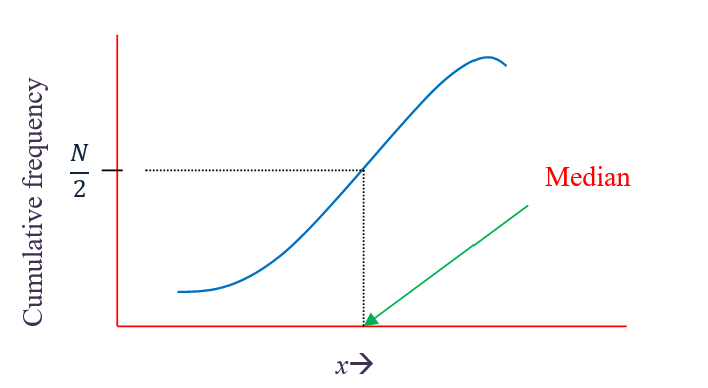
Figure 3.1: median from a cumulative frequency curve
Example 3.7 Table below gives the distribution of the heights of 60 students in a Senior High school. Find the median height of the students
| Height(cm) | 145-150 | 150-155 | 155-160 | 160-165 | 165-170 | 170-175 |
|---|---|---|---|---|---|---|
| Number of students | 3 | 9 | 16 | 18 | 10 | 4 |
Solution 3.7
(i) Linear interpolation method for estimating the median
\(N\) = 60
Median class= class interval which contains the \(\left( \frac{N}{2} \right)^{\text{th}}\)ordered observation; here \(\left( \frac{60}{2} \right)^{\text{th}} =\) 30th observation. Before the class 160-165 there are 3+9+16=28 observations so 30th observation will be in the class 160-165, therefore it is the median class.
\(L\) = lower limit of the median class =160
\(F\) = sum of all frequencies below 160(cumulative frequency) = 16+9+3= 28
\(f_{m}\) = frequency of the median class=18
\(C\) = class width of the median class=5
\(median = 160 + \left( \frac{\frac{1}{2}60 - 28}{18} \right)5\) = 160.56
(ii) Estimation of the median from a cumulative frequency curve
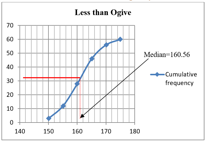
Figure 3.2: Median from a cumulative frequency curve Example 3.7
3.2.4 Merits and Demerits of Median
Merits
Median is not influenced by extreme values because it is a positional average.
Median can be calculated in case of distribution with open-end intervals.
Median can be located even if the data are incomplete.
Demerits
A slight change in the series may bring drastic change in median value.
In case of even number of items or continuous series, median is an estimated value other than any value in the series.
It is not suitable for further mathematical treatment except its use in calculating mean deviation.
It does not take into account all the observations.
3.3 The mode
The mode of a set of data is the value which occurs with the greatest frequency. The mode is therefore the most common value. The mode is an important measure in case of qualitative data. The mode can be used to describe both quantitative and qualitative data.
3.3.1 Mode of ungrouped or raw data
For ungrouped data or a series of individual observations, mode is often found by mere inspection.
Example 3.8
\(a)\) The modes of 1, 2, 2, 2, 3 is 2.
\(b)\) The modes of 2, 3, 4, 4, 5, 5 are 4 and 5.
\(c)\) The mode does not exist when every observation has the same frequency. For example, the following sets of data have no modes: (i) 3, 6, 8, 9; (ii) 4, 4, 4, 7, 7, 7, 9, 9, 9.
Note: It can be seen that the mode of a distribution may not exist, and even if it exists, it may not be unique. Distributions with a single mode are referred to as unimodal. Distributions with two modes are referred to as bimodal. Distributions may have several modes, in which case they are referred to as multimodal.
Example 3.9 20 patients selected at random had their blood groups determined. The results are given in the table below
| Blood group | A | AB | B | O |
|---|---|---|---|---|
| No. of patients | 2 | 4 | 6 | 8 |
The blood group with the highest frequency is O. The mode of the data is therefore blood group O. We can say that most of the patients selected have blood group O. Notice that the mean and the median cannot be applied to the data. This is because the variable “blood group” cannot take numerical values. However, it can be seen that the mode can be used to describe both quantitative and qualitative data.
3.3.2 Mode of Grouped frequency distribution
\[mode = L + \left( \frac{f_{m}-f_{p}}{2f_{m}-f_{p} - f_{s}} \right)C\]
Locate the highest frequency the class corresponding to that frequency is called the modal class.
Where \(L\) = lower limit of the modal class; \(f_{m}\) = the frequency of modal class; \(f_{p}\)= the frequency of the class preceding the modal class; \(f_{s}\)= the frequency of the class succeeding the modal class and \(C\) = class interval
Example 3.10 For the frequency distribution of weights of sorghum ear-heads given in table below. Calculate the mode.
| Weights of ear heads (g) | No of ear heads (f) |
|---|---|
| 60-80 | 22 |
| 80-100 | 38 |
| 100-120 | 45 |
| 120-140 | 35 |
| 140-160 | 20 |
Modal class is 100-120
\(mode = 100 + \left( \frac{45-35}{90-38-35} \right)20 =\) 111.76
3.3.3 Mode using Histogram
Consider the figure below. The modal class is the class interval which corresponds to rectangle \(\text{ABCD}\). An estimate of the mode of the distribution is the abscissa of the point of intersection of the line segments \(\overline{\text{AE}}\) and \(\overline{\text{BF}}\) in the figure.

Figure 3.3: Median from a cumulative frequency curve for Example 3.10
3.3.4 Merits and Demerits of Mode
Merits
It is readily comprehensible and easy to compute. In some case it can be computed merely by inspection.
It is not affected by extreme values. It can be obtained even if the extreme values are not known.
Mode can be determined in distributions with open classes.
Mode can be located on the graph also.
Mode can be used to describe both quantitative and qualitative data.
Demerits
The mode is not unique. That is, there can be more than one mode for a given set of data.
The mode of a set of data may not exist.
It is not based upon all the observation.