5 Measures of Dispersion
We discussed in previous chapters, how a set of data can be summarized
by a single representative value which describes the central value of
the data. Consider the two sets of data A & B below
| Data sets | ||||||
|---|---|---|---|---|---|---|
| A | 1 | 2 | 3 | 3 | 4 | 5 |
| B | -1 | 0 | 3 | 3 | 5 | 8 |
You can see mean, median and mode for both the sets A & B is 3
See the dot diagrams of data sets A and B.
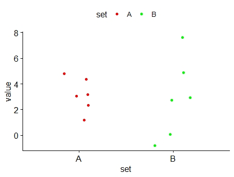
Figure 5.1: Scatter diagram of data sets A & B
It can be seen that, while values of data set A are grouped close to their mean, while the values of data set B are more spread out. We say that values of data set B are more dispersed (or scattered) than those of data set A
This example shows that the mean, the mode and the median, are not enough in describing a set of data. In addition to using these measures, we need a numerical measure of dispersion (or variation) of a set of data.
Statistical dispersion means the extent to which a numerical data is likely to vary about an average value.
5.1 Characteristics of a good measure of dispersion
An ideal measure of dispersion is expected to possess the following properties
It should be rigidly defined.
It should be based on all the items.
It should not be unduly affected by extreme items.
It should lend itself for algebraic manipulation.
It should be simple to understand and easy to calculate.
The most important measures of dispersion are Range, Quartile deviation, Variance, Inter-quartile range, Mean Absolute Deviation (MAD)and standard deviation.
5.2 The Range
This is the simplest possible measure of dispersion. The range of a set of data is defined as the difference between the largest observation and the smallest observation in the set of data.
Thus,
Range = largest observation – smallest observation.
In symbols, Range = L – S.
Where L = Largest value; S = Smallest value.
In individual observations and discrete series, L and S are easily identified. In continuous series, the following two methods are followed.
5.2.1 Method 1
L = Upper boundary of the highest class
S = Lower boundary of the lowest class.
\[Range = L - S\]
Example 5.1: The marks obtained by 8 students in Mathematics and Physics examinations are as follows:
Mathematics: 35, 60, 70, 40, 85, 96, 55, 65.
Physics: 50, 55, 70, 65, 89, 68, 72, 80.
Find the ranges of the two sets of data. Are the Physics marks more dispersed than the Mathematics marks?
Solution
For Mathematics,
Highest mark = 96, lowest mark = 35, range =96 – 35 = 61
For Physics,
Highest mark = 89, lowest mark = 50, range =89 – 50 = 39.
The mathematics marks have a wider range than the Physics marks. The Mathematics marks are therefore more dispersed than the Physics marks.
Example 5.2: Calculate range from the following distribution
| Size | 60-63 | 63-66 | 66-69 | 69-72 | 72-75 |
|---|---|---|---|---|---|
| Number | 5 | 18 | 42 | 27 | 8 |
Solution
L = Upper boundary of the highest class = 75
S = Lower boundary of the lowest class = 60
Range = L – S = 75 – 60 = 15
5.2.2 Merits and Demerits of Range
Merits
It is simple to understand.
It is easy to calculate.
In certain types of problems like quality control, weather forecasts, share price analysis, etc.
Demerits
It is very much affected by the extreme items.
It is based on only two extreme observations.
It cannot be calculated from open-end class intervals.
It is not suitable for mathematical treatment.
It is a very rarely used measure.
5.3 The Inter-Quartile Range (IQR) or Midspread
The range has the advantage that it is quick and easy to calculate. However, since it depends only on the maximum and the minimum values of a set of data, it does not show how the whole data is distributed between these two values. The range is therefore not a good measure of dispersion if one or both of these two values differ greatly from other values of the data. To overcome this problem, we sometimes use the inter-quartile range. A robust measure of dispersion is the inter-quartile range. The inter-quartile range of a set of data is the difference between the upper and lower quartiles of the data. Thus,
\[Inter-Quartile Range (IQR) = Q_3 - Q_1\]
The inter-quartile range of a set of data is therefore not affected by values of the data outside Q1 and Q3. The inter-quartile range is sometimes used as a measure of dispersion.
Example 5.3: Consider the two sets of data below, find IQR
A: 3, 4, 5, 6, 8, 9, 10, 12, 15
B: 3, 8, 8, 9, 9, 9, 10, 10, 15
For data set A, Q1 = 4.5, Q3 = 11; so Inter-Quartile Range =11 – 4.5 = 6.5
For data set B, Q1 = 8, Q3 = 10; so Inter-Quartile Range =10 – 8 = 2
Since the inter-quartile range of data set A is greater than that of data set B, these results confirm that data set A is more dispersed than data set B. You can also see Range is same for both the sets.
5.4 Mean Absolute Deviation (MAD)
The mean absolute deviation (MAD) is a measure of variability that indicates the average distance between observations and their mean. MAD uses the original units of the data, which simplifies interpretation. Larger values signify that the data points spread out further from the average. Conversely, lower values correspond to data points bunching closer to it. The mean absolute deviation is also known as the mean deviation and average absolute deviation.
Here is how to calculate the mean absolute deviation.
Calculate the mean.
Calculate the difference of each observation from mean and take absolute value i.e. ignore the sign. This difference is known as absolute deviation
Add those deviations together.
Divide the sum by the number of data points.
\[MAD = \frac{\sum_{i = 1}^{n}\left| x_{i} - \overline{x} \right|}{n}\]
Example 5.4: find the mean absolute deviation of the following 10, 15, 15, 17, 18, 21
| Sl.No. | \[x_{i}\] | \[x_{i} - \overline{x}\] | \[\left| x_{i} - \overline{x} \right|\] |
|---|---|---|---|
| 1 | 10 | -6 | 6 |
| 2 | 15 | -1 | 1 |
| 3 | 15 | -1 | 1 |
| 4 | 17 | 1 | 1 |
| 5 | 18 | 2 | 2 |
| 6 | 21 | 5 | 5 |
| \(\overline{x} =\) 16 | \(\sum_{i = 1}^{n}\left| x_{i} - \overline{x} \right|\) = 16 |
Here n = 6 and \(\sum_{i = 1}^{n}\left| x_{i} - \overline{x} \right|\) = 16 therefore MAD = \(\frac{16}{6} = 2.67\)
5.4.1 Merits and Demerits of MAD
Merits
Mean deviation is simple and easy.
Different items of observations can be easily compared with mean deviation.
Mean deviation is better than quartile deviation and range because it is based on all the observations of the series.
Mean deviation is less affected by the extreme values in the series while comparing to standard deviation.
Mean deviation is rigidly defined. So, it has fixed value.
Mean deviation about median will be least.
Demerits
Mean deviation becomes difficult to compute mean deviation in case of fractions.
It is not applicable for algebraic calculations.
It cannot be calculated from open-end class intervals.
Mean deviation is not a good measure as it ignores negative signs of deviations.
5.5 The variance and standard deviation
The most important measures of variability are the sample variance and the sample standard deviation. If x1, x2… xn is a sample of n observations, then the sample variance is denoted by s² and is defined by the equation.
\[{\mathbf{\text{sample variance}},\ \mathbf{s}}^{\mathbf{2}}\mathbf{=}\frac{\sum_{\mathbf{i = 1}}^{\mathbf{n}}\left( \mathbf{x}_{\mathbf{i}}\mathbf{-}\overline{\mathbf{x}} \right)^{\mathbf{2}}}{\mathbf{n - 1}}\]
The sample standard deviation, s, is the positive square root of the sample variance.
\[\mathbf{variance =}\left( \mathbf{\text{standard deviation}} \right)^{\mathbf{2}}\]
\[\mathbf{standard\ deviation = \ }\sqrt{\mathbf{\text{variance}}}\]
Note: If sA, the standard deviation of data set A, is greater than sB, the standard deviation of data set B, then data set A is more dispersed than data set B. It should be noted that the standard deviation of a set of data is a non-negative number.
Example 5.4: Consider the two sets of data A & B below; find standard deviation?
| A | 1 | 2 | 3 | 3 | 4 | 5 |
|---|---|---|---|---|---|---|
| B | -1 | 0 | 3 | 3 | 5 | 8 |
Solution:
| Set A | |||
|---|---|---|---|
| \[\mathbf{x}_{\mathbf{i}}\] | \[\left(\mathbf{x}_{\mathbf{i}}\mathbf{-}\overline{\mathbf{x}}\right)\] | \[\left(\mathbf{x}_{\mathbf{i}}\mathbf{-}\overline{\mathbf{x}}\right)^{\mathbf{2}}\] | |
| 1 | -2 | 4 | |
| 2 | -1 | 1 | |
| 3 | 0 | 0 | |
| 3 | 0 | 0 | |
| 4 | 1 | 1 | |
| 5 | 2 | 4 | |
| Sum | 18 | 0 | 10 |
Mean (\(\overline{x}\)) =\(\ \frac{18}{6} = 3\)
\[{sample\ variance,\ s}_{A}^{2} = \frac{\sum_{i = 1}^{n}\left( x_{i} - \overline{x} \right)^{2}}{n - 1} = \frac{10}{5} = 2\]
\[\text{sample standard deviation,}\ s_{A} = \ \sqrt{s_{A}^{2}} = \ \sqrt{2} = 1.414\]
| Set B | |||
|---|---|---|---|
| \[\mathbf{x}_{\mathbf{i}}\] | \[\left( \mathbf{x}_{\mathbf{i}}\mathbf{-}\overline{\mathbf{x}} \right)\] | \[\left( \mathbf{x}_{\mathbf{i}}\mathbf{-}\overline{\mathbf{x}} \right)^{\mathbf{2}}\] | |
| -1 | -4 | 16 | |
| 0 | -3 | 9 | |
| 3 | 0 | 0 | |
| 3 | 0 | 0 | |
| 5 | 2 | 4 | |
| 8 | 5 | 25 | |
| Sum | 18 | 0 | 54 |
Mean (\(\overline{x}\)) =\(\ \frac{18}{6} = 3\)
\[{Sample\ variance,\ s}_{B}^{2} = \frac{\sum_{i = 1}^{n}\left( x_{i} - \overline{x} \right)^{2}}{n - 1} = \frac{54}{5} = 10.8\]
\[Sample\ standard\ deviation,\ s_{B} = \ \sqrt{s_{B}^{2}} = \ \sqrt{10.8} = 3.29\]
It can be seen that \(s_{B} > s_{A}\), confirming that data set B is more dispersed than data set A (see the dot diagrams)
Note: The unit of measurement of the sample variance is the square of the unit of measurement of the data. Sample standard deviation has same unit of measurement as of the data. Thus, if x is measured in centimetres (cm), then the unit of measurement of the sample variance is cm2 and that of sample standard deviation is cm. The standard deviation has the desirable property of measuring variability in the same unit as the data.
An alternative formula for computing the variance
The computation of s² requires calculations of \(\overline{x}\), n subtractions and n squaring and adding operations. If the original observations or the deviations \(\left( x_{i} - \overline{x} \right)\) are not integers, the deviations \(\left( x_{i} - \overline{x} \right)\) may be difficult to work with, and several decimals may have to be carried to ensure numerical accuracy. A more efficient computational formula for s² is given by
\(s^{2} = \frac{1}{n - 1}\left\{ \sum_{i = 1}^{n}{x_{i}^{2} - \frac{1}{n}}\left( \sum_{i = 1}^{n}x_{i} \right)^{2} \right\}\)
Example 5.5: Consider the data set below; find standard deviation?
| 3 | 4 | 5 | 6 | 8 | 9 | 10 | 12 | 15 |
Solution:
| \[\mathbf{x}_{\mathbf{i}}\] | \[\mathbf{x}_{\mathbf{i}}^{\mathbf{2}}\] | |
|---|---|---|
| 3 | 9 | |
| 4 | 16 | |
| 5 | 25 | |
| 6 | 36 | |
| 8 | 64 | |
| 9 | 81 | |
| 10 | 100 | |
| 12 | 144 | |
| 15 | 225 | |
| Sum | 72 | 700 |
\(s^{2} = \frac{1}{n - 1}\left\{ \sum_{i = 1}^{n}{x_{i}^{2} - \frac{1}{n}}\left( \sum_{i = 1}^{n}x_{i} \right)^{2} \right\}\) ; here n = 9
\(s^{2} = \frac{1}{8}\left\{ 700 - {\frac{1}{9}\left( 72 \right)}^{2} \right\}\) =15.5
\(s = \ \sqrt{15.5} = 3.94\)
5.5.1 Variance and standard deviation for grouped data
5.5.1.1 For discrete grouped data
\[s^{2} = \frac{1}{n - 1}\left\{ \sum_{i = 1}^{n}{{f_{i}x}_{i}^{2} - \frac{1}{n}}\left( \sum_{i = 1}^{n}{f_{i}x}_{i} \right)^{2} \right\}\]
where \(f_{i}\) is the frequency of ith observation
Example 5.6: The frequency distributions of seed yield of 50 sesamum plants are given below. Find the standard deviation.
| Seed yield in gms (x) | 3 | 4 | 5 | 6 | 7 |
|---|---|---|---|---|---|
| Frequency (f) | 4 | 6 | 15 | 15 | 10 |
Solution:
| x | f | fx | fx2 |
|---|---|---|---|
| 3 | 4 | 12 | 36 |
| 4 | 6 | 24 | 96 |
| 5 | 15 | 75 | 375 |
| 6 | 15 | 90 | 540 |
| 7 | 10 | 70 | 490 |
| Total | 50 | 271 | 1537 |
\[s^{2} = \frac{1}{n - 1}\left\{ \sum_{i = 1}^{n}{{f_{i}x}_{i}^{2} - \frac{1}{n}}\left( \sum_{i = 1}^{n}{f_{i}x}_{i} \right)^{2} \right\}\]
\[{sample\ variance,\ s}^{2} = \frac{1}{50 - 1}\left\{ 1537 - \frac{271^{2}}{50} \right\} = 1.3914\]
\(standard\ deviation,\ s = \sqrt{1.3914}\) = 1.179
5.5.1.2 For continuous grouped data
\[s^{2} = \frac{1}{n - 1}\left\{ \sum_{i = 1}^{n}{{f_{i}d}_{i}^{2} - \frac{1}{n}}\left( \sum_{i = 1}^{n}{f_{i}d}_{i} \right)^{2} \right\}\]
where \(f_{i}\) is the frequency of ith class, c is the class interval, \(d_{i} = \frac{x_{i} - A}{c}\), \(x_{i}\) is the class mark, \(A\) is the class mark with the highest frequency
Example 5.7: The frequency distributions of seed yield of 50 sesamum plants are given below. Find the standard deviation
| Seed yield in gms (x) | 2.5-3.5 | 3.5-4.5 | 4.5-5.5 | 5.5-6.5 | 6.5-7.5 |
|---|---|---|---|---|---|
| Frequency (f) | 4 | 6 | 15 | 15 | 10 |
Solution:
Here n =50; c =1
| Seed yield | f | x | \[d_{i} = \frac{x_{i} - A}{c}\] | fd | f d2 |
|---|---|---|---|---|---|
| 2.5-3.5 | 4 | 3 | -2 | -8 | 16 |
| 3.5-4.5 | 6 | 4 | -1 | -6 | 6 |
| 4.5-5.5 | 15 | 5 | 0 | 0 | 0 |
| 5.5-6.5 | 15 | 6 | 1 | 15 | 15 |
| 6.5-7.5 | 10 | 7 | 2 | 20 | 40 |
| Total | 50 | 25 | 0 | 21 | 77 |
A = 5
\[s^{2} = \frac{1}{n - 1}\left\{ \sum_{i = 1}^{n}{{f_{i}d}_{i}^{2} - \frac{1}{n}}\left( \sum_{i = 1}^{n}{f_{i}d}_{i} \right)^{2} \right\}\]
\[{sample\ variance,\ s}^{2} = \frac{1}{49}\left( 77 - \frac{\left( 21 \right)^{2}}{50} \right) = \ 1.3914\]
\(standard\ deviation,\ s = \sqrt{1.3914}\) = 1.179
5.5.2 Merits and Demerits of Standard Deviation
Merits
It is rigidly defined and its value is always definite and based on all the observations.
As it is based on arithmetic mean, it has all the merits of arithmetic mean.
It is the most important and widely used measure of dispersion.
It is possible for further algebraic treatment.
It is less affected by the fluctuations of sampling and hence stable.
It is the basis for measuring the coefficient of correlation and other measures.
Demerits
It is not easy to understand and it is difficult to calculate.
It gives more weight to extreme values because the values are squared up.
As it is an absolute measure of variability, it cannot be used for the purpose of comparison.
5.6 Coefficient of Variation (relative measure of dispersion)
The Standard deviation is an absolute measure of dispersion. It is expressed in terms of units in which the original figures are collected and stated. The standard deviation of heights of plants cannot be compared with the standard deviation of weights of the grains, as both are expressed in different units, i.e heights in centimetre and weights in kilograms.
Therefore the standard deviation must be converted into a relative measure of dispersion for the purpose of comparison. The relative measure is known as the coefficient of variation. The coefficient of variation is obtained by dividing the standard deviation by the mean and expressed in percentage.
\[\mathbf{\text{Coefficient of variation}}\left( \mathbf{C}\mathbf{.}\mathbf{V} \right)\mathbf{=}\frac{\mathbf{\text{standard deviation}}}{\mathbf{\text{mean}}}\mathbf{\times 100}\]
If we want to compare the variability of two or more series, we can use C.V. The series or groups of data for which the C.V. is greater indicate that the group is more variable, less stable, less uniform, less consistent or less homogeneous. If the C.V. is less, it indicates that the group is less variable or more stable or more uniform or more consistent or more homogeneous.
Example 5.8: Consider the measurement on yield and plant height of a paddy variety. The mean and standard deviation for yield are 50 kg and 10 kg respectively. The mean and standard deviation for plant height are 55 cm and 5 cm respectively. Compare the variability.
Solution:
Here the measurements for yield and plant height are in different units. Hence the variability can be compared only by using coefficient of variation.
For yield, CV=\(\ \frac{10}{50} \times 100 =\) 20%
For plant height, CV= \(\frac{5}{55} \times 100 =\) 9.1%
The yield is subject to more variation than the plant height.