10 Probability Distributions
10.1 Random experiment
A random experiment is an experiment or a process for which the outcome cannot be predicted with certainty. The sample space (denoted S) of a random experiment is the set of all possible outcomes.
Example: Tossing a coin, Throwing a die etc
10.2 Random variable
A Random Variable is a set of possible values from a random experiment. Random variable is usually denoted as ‘\(X\)’
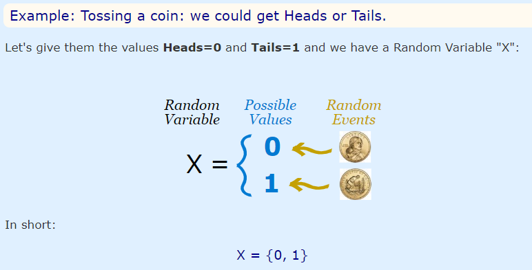
Figure 10.1: Tossing a coin
A random variable has a whole set of values and it could take on any of those values, randomly. Not like an Algebra Variable, In Algebra a variable, like X, is an unknown value. But a random variable is different.
Probability of a random variable can be represented by \(p(X = x)\) or \(p(x)\).Small letter \(x\) denotes the value taken by the random variable \(X\).
For example throwing a die once
Here you can define a random variable of your interest. Defining a random variable is like:
Let \(X\) be the number appearing on throwing the dice then; \(x\) = {1, 2, 3, 4, 5, 6}. The random variable \(X\) can take any values shown above. In this case they are equally likely, probability of anyone is 1/6. So, \(p(X = x)\) = \(p(x)\) =1/6
Let \(X\) be the even number appearing on throwing the dice then; \(X\) = {2, 4, 6}. The random variable \(X\) can take any values shown above. \(p(X = x)\) = \(p(x)\) = 3/6
10.3 Probability distributions
A probability distribution is a list of all of the possible outcomes of a random variable along with their corresponding probability values.
Example: - Tossing a coin 3 times
Defining random variable:
Let X be the number of heads appearing on throwing the dice In this case there would be 0 heads, 1, 2 and 3 heads, so the sample space is \(X\) = {0, 1, 2, 3} and they are not equally likely.
There are total 8 possible cases on tossing coin three times is shown in table below
| On tossing thrice | No: of heads (\(X\)) |
|---|---|
| HHH | 3 |
| HHT | 2 |
| HTH | 2 |
| THH | 2 |
| HTT | 1 |
| THT | 1 |
| TTH | 1 |
| TTT | 0 |
\(p(X = x)\) = \(\frac{No: \ of \ times\ X\ takes\ value\ x}{8}\)
\(p(X = 3)\) = 1/8; \(p(X = 2)\) = 3/8; \(p(X = 1)\) = 3/8; \(p(X = 0)\) = 1/8
A probability distribution is a list of all of the possible outcomes of a random variable along with their corresponding probability values.
Table below shows a probability distribution.
| \(X\) | \(p(x)\) |
|---|---|
| 0 | 1/8 |
| 1 | 3/8 |
| 2 | 3/8 |
| 3 | 1/8 |
This is an example of discrete probability distribution as \(X\) takes only discrete values. If \(x\) takes continuous values, it is termed as continuous probability distribution.
10.4 Probability mass function
When we use a probability function to describe a discrete probability distribution, we call it a probability mass function (commonly abbreviated as p.m.f). A probability mass function, returns the probability of an outcome. Therefore, a probability mass function is written as: \(p(x)\) = \(p(X = x)\). Here the variable \(X\) is discrete in nature.
10.5 Probability density function
When we use a probability function to describe a continuous probability distribution, we call it a probability density function (commonly abbreviated as p.d.f).
10.6 Expected value of a random variable
Expected value is exactly what you might think it means. The return you
can expect for some kind of action. The expected value of a random
variable is the long-run average value of repetitions of the same
experiment it represents. For example, the expected value in rolling a
six-sided die is 3.5, because the average of all the numbers that come
up is 3.5 as the number of rolls approaches infinity. Expected value of
random variable \(X\) is denoted as \(E(X)\).
The formula for calculating the Expected Value of random variable where
there are multiple probabilities is
E(\(X\)) = \(\sum_{i = 1}^{\infty}xp(x)\) (discrete case)
E(\(X\)) = \(\int_{- \infty}^{\infty}{x p(x)\ \text{dx }}\) (continuous case); \(- \infty \leq x \leq \infty\)
here the random variable \(X\) lies between \({-\infty}\) and \({+\infty}\)
Example
- Find Expected value of \(X\) of tossing a single unfair die
| x | 1.0 | 2.0 | 3.0 | 4.0 | 5.0 | 6.0 |
| p(x) | 0.1 | 0.1 | 0.1 | 0.1 | 0.1 | 0.5 |
Solution:
| xp(x) | 0.1 | 0.2 | 0.3 | 0.4 | 0.5 | 3 |
E(\(X\)) = \(\sum_{i = 1}^{6}xp(x)\)
= 0.1+0.2+0.3+0.4+0.5+3 = 4.5
- Find E(X) in the following case (Practice question)
| \(x\) | \(p(x)\) |
|---|---|
| 0 | 1/8 |
| 1 | 3/8 |
| 2 | 3/8 |
| 3 | 1/8 |
10.7 Discrete probability distributions
We have seen that a probability distribution is a list of all of the possible outcomes of a random variable along with their corresponding probability values. It is represented as a table. It will be more convenient if it can be expressed as an equation. So if the value of x is given we can calculate the corresponding probability from the equation. There are several discrete distributions depending on situations. Our discussion is limited to following discrete distributions.
Bernoulli distribution
Binomial distribution
Poisson distribution
10.7.1 Bernoulli distribution
A Bernoulli distribution is a discrete probability distribution. This distribution applies to random experiment that has only two outcomes (usually called a “Success” or a “Failure”).
For example tossing a coin has only two outcomes which can be termed as success and failure by the experimenter
Success: getting head
Failure: getting tail
The probability mass function of the distribution is
\(p(X = x)\) = \(p(x)\) = \(p\)\(x\) \((1-p)\)\(1-x\), where \(X\) takes only two values = 0,1
The expected value for a random variable, \(X\), from a Bernoulli distribution is: E(\(X\)) = \(p\) and the variance of a Bernoulli random variable is: var(\(X\)) = \(p(1 - p)\).
Example
Find the probability assuming Bernoulli distribution of a biased coin where probability of success (getting head) \(p\) = 0.4
Let \(X\) be the random variable which takes value 0 on getting tail (failure) and takes value 1 on getting head (success). So using the equation
p(\(X\) = \(x\)) = p(\(X\)) = p\(X\) \((1-p)\)\(1-x\)
P(\(X\) = 0) = (0.4)0(1-0.4)1 =0.6
P(\(X\) = 1) = (0.4)1(1-0.4)0 =0.4
| \(x\) | \(p(x)\) |
|---|---|
| 0 | 0.6 |
| 1 | 0.4 |
A Bernoulli trial is one of the simplest experiments you can conduct in probability and statistics. It’s an experiment where you can have one of two possible outcomes. For example, “Yes” and “No” or “Heads” and “Tails.”
10.7.2 Binomial distribution
Binomial distribution can be thought of as simply the probability of a SUCCESS or FAILURE outcome in an experiment or survey that is repeated multiple times; i.e. a Binomial distribution happens, when a Bernoulli trial is repeated \(n\) number of times. The binomial is a type of distribution that has two possible outcomes (the prefix “bi” means two, or twice). For example when a coin toss is repeated 5 times, the random variable, \(X\) = no: of heads will follow a binomial distribution with \(n\) = 5.
Binomial distributions must also meet the following three criteria:
The number of observations or trials is fixed. (\(n\))
Each observation or trial is independent
The probability of success (tails, heads, fail or pass) is exactly the same from one trial to another (\(p\))
The probability mass function of the distribution is
\(p(x)\) = nCx\(p^x\) \(q^{n-x}\) = \(\frac{n!}{\left( n - x \right)!x!\ }\) \(p^x\) \(q^{n-x}\)
where x takes values = 0,1,2,..., \(n\)
\(n\)= number of trials
\(x\)= number of success desired
\(p\)= probability of getting a success in one trial
\(q\) = \(1-p\) = probability of getting a failure in one trial
E(\(X\)) = \(np\)
V(\(X\)) = \(npq\); \(n\) and \(p\) are the most important parameters in binomial distribution.
Mean of binomial distribution is \(np\) and variance is \(npq\)
Example
A coin is tossed 10 times. What is the probability of getting exactly 6 heads?
here,
\(n\) = 10
\(x\) = 6
\(p\) = ½
\(q\) = \(1-p\) = ½
We have to find \(p(X=6)\); using the formula \(p(X=x)\) \(=\) nCx\(p^x\) \(q^{n-x}\)
\(p(X=6)\) = 10\(c\)6\(\left( \frac{1}{2} \right)^{6}\left( \frac{1}{2} \right)^{10 - 6}\)= 0.2050
10.7.3 Poisson distribution
Discovered by the French Mathematician Simeon Denis Poisson (1781 -1840). It is developed to describe the number of times a gambler would win a rarely won game of chance in a large number of tries, i.e. Poisson distribution deals with rare events.
Poisson distribution is first applied to study the number of death by horse kicking in the Prussian army.
Other applications and examples where Poisson distribution is used
Pest incidence
Birth defects and genetic mutations
Rare diseases
Car accidents
Traffic flow and ideal gap distance
Number of typing errors on a page
Hairs found in McDonald’s hamburgers
Spread of an endangered animal in Africa
Failure of a machine in one month
A random variable \(X\) is said to follow a Poisson distribution; if it assumes non-negative values and its probability mass function is given by:
\[p\left( X = x \right) = \frac{e^{- \lambda}.\lambda^{x}}{x!}\]
where \(x\) = 0,1,2,… ., ∞,
\(e\) = 2.7183.
\(λ\) : Average number of successes occurring in a given time interval or region in the Poisson distribution
It is a discrete distribution with a single parameter λ
The mean and the variance of the Poisson distribution are both equal to \(λ\)
Example
The average number of homes sold by a Realty company is 2 homes per day. Assuming Poisson distribution what is the probability that exactly 3 homes will be sold tomorrow?
Solution:
\(λ\) = 2; since 2 homes are sold per day, on average.
\(x\) = 3; since we want to find the probability that 3 homes will be sold tomorrow.
\(e\) = 2.71828; since e is a constant equal to approximately 2.71828.
\[p\left( X = x \right) = \frac{e^{- \lambda}.\lambda^{x}}{x!}\]
\(p(X=3)\) = \(\ \frac{{2.71828}^{- 2}{\ \times \ 2}^{3}}{3!}\)
\(p(X = 3)\) = 0.180
Questions
If the random variable X follows a Poisson distribution with mean 3.4, find \(p(X = 6)\)
The number of industrial injuries per working week in a particular factory is known to follow a Poisson distribution with mean 0.5. Find the probability that in a particular week there will be:
\(i)\) Less than 2 accidents \[Hint: p(X<2) = p(X = 0) + p(X = 1)\]
\(ii)\) More than 2 accidents \[Hint: p(X>2) = 1-{p(X = 0) + p(X = 1) + p(X =2)}\]
- A company known on the past experience that 3% of the bulbs they
produced are defective. Assuming Poisson distribution find the
probability of getting the following in a sample of 100 bulbs:
\[Hint: here \ λ = n × p = 100 × 0.03\]
No defective \[Hint: let X be the number of defectives; x = 0\]
1 defective \[Hint: x = 1\]
2 defectives \[Hint: x = 2\]
3 defectives\[Hint: x = 3\]
Distributions Bernoulli, Binomial and Poisson that we discussed so far are discrete distributions.
10.8 Continuous probability distributions
If the random variable X is continuous, the corresponding probability distribution is termed as continuous probability distribution. There are several continuous distributions. Our discussion is limited to only Normal distribution.
10.8.1 Normal distribution
The normal distribution is defined by the following probability density function (probability density function is explained in above section)
\[f\left( x \right) = \frac{1}{\sqrt{2\pi\sigma}}e^{- \frac{{(x - \mu)}^{2}}{2\sigma^{2}}}\]
, where \(- \infty < x < + \infty\) ; \(μ\) is the population mean and \(σ\)2 is the variance, e = 2.718.
If a random variable \(X\) follows the normal distribution, then we write:
\(X\)~\(N\)(\(μ\), \(σ\)2)
In particular, the normal distribution with \(μ\) = 0 and \(σ\)2 = 1 is called the standard normal distribution, and is denoted as \(X\)~\(N\)(0,1).
Properties of Normal distribution
The normal distribution is the most frequently used among all probability laws. The normal distribution can be found in many practical problems.
If you plot density \(f(x)\) against \(x\) the graph will be bell shaped always
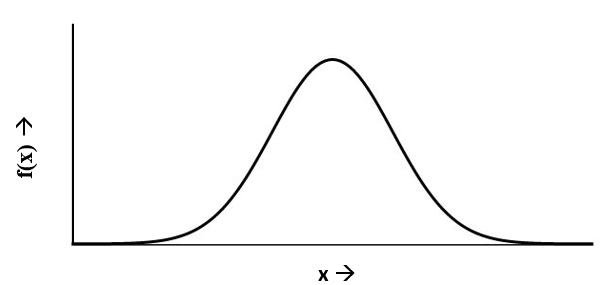
Figure 10.2: Normal distribution curve
Many things closely follow a Normal Distribution:
Yield of crops
heights of people
size of things produced by machines
errors in measurements
blood pressure
marks on a test
The Normal Distribution has:
mean = median = mode
Mean is located to the centre of the curve. mean = median = mode, all these locate towards the centre
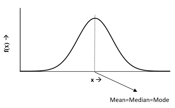
Figure 10.3: Mean=Median=Mode in normal distribution
Normal distribution is symmetric about the centre, 50% of values less than the mean and 50% greater than the mean
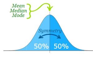
Figure 10.4: Normal distribution is a symmetric distribution
10.8.1.1 Standardisation of Normal distribution
The standard normal distribution is a special case of the normal distribution where the mean is zero and the standard deviation is 1.
This distribution is also known as the Z-distribution. A value on the standard normal distribution is known as a standard score or a Z-score.
A standard score or Z-score represents the number of standard deviations above or below the mean that a specific observation falls.
So to convert a value to a Standard Score (“z-score”):
First subtract the mean,
Then divide by the Standard Deviation
And doing that is called “Standardizing”.
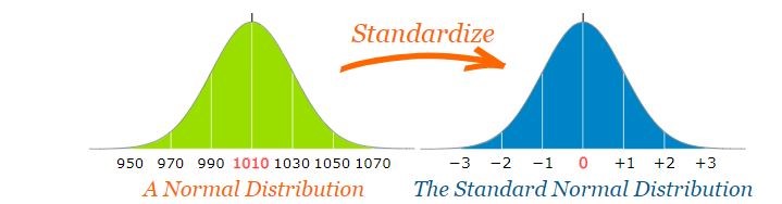
Figure 10.5: Standardization of Normal distribution
Example: A survey of daily travel time had these results (in minutes):
\(X\): 26, 33, 65, 28, 34, 55, 25, 44, 50, 36, 26, 37, 43, 62, 35, 38, 45, 32, 28, 34
Convert it in to standard scores (Z-score).
The Mean is 38.8 minutes, and the Standard Deviation is 11.4
First subtract the mean from observation
Then divide by the Standard Deviation
| \(X\) | \(X-\mu\) | \[z = \frac{X - \mu}{\sigma}\] |
|---|---|---|
| 26 | -12.8 | -1.12 |
| 33 | -5.8 | -0.51 |
| 65 | 26.2 | 2.30 |
| 28 | -10.8 | -0.95 |
| 34 | -4.8 | -0.42 |
| 55 | 16.2 | 1.42 |
| 25 | -13.8 | -1.21 |
| 44 | 5.2 | 0.46 |
| 50 | 11.2 | 0.98 |
| 36 | -2.8 | -0.25 |
| 26 | -12.8 | -1.12 |
| 37 | -1.8 | -0.16 |
| 43 | 4.2 | 0.37 |
| 62 | 23.2 | 2.04 |
| 35 | -3.8 | -0.33 |
| 38 | -0.8 | -0.07 |
| 45 | 6.2 | 0.54 |
| 32 | -6.8 | -0.60 |
| 28 | -10.8 | -0.95 |
| 34 | -4.8 | -0.42 |
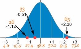
Figure 10.6: Z score values for X
The z-score formula that we have been using is:
\[z = \frac{x - \mu}{\sigma}\]
z is the “z-score” (Standard Score)
\(x\) is the value to be standardized
\(μ\) (’mu”) is the mean
\(σ\) (“sigma”) is the standard deviation
Parameters of Normal distribution
As with any probability distribution, the parameters of the normal distribution define its shape and probabilities entirely. The normal distribution has two parameters, mean (\(μ\)) and standard deviation (\(σ\)). The normal distribution does not have just one form. Instead, the shape changes based on the parameter values.
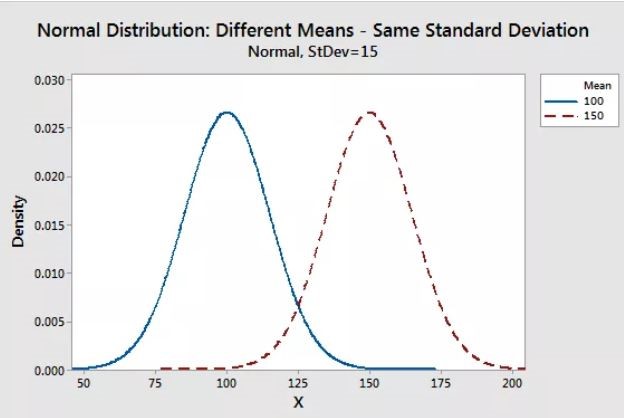
Figure 10.7: Shape changes in normal distribution based on different means
Standard deviation:
The standard deviation is a measure of variability. It defines the width of the normal distribution. It determines how far away from the mean the values tend to fall. It represents the typical distance the observations and the average.
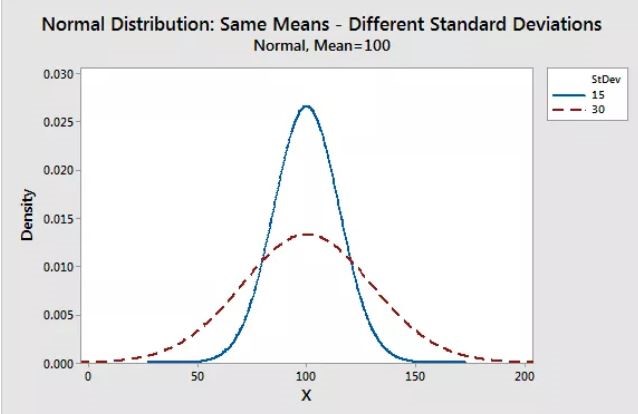
Figure 10.8: Shape changes in normal distribution based on different standard deviation
When you have normally distributed data, the standard deviation can be used to determine the proportion of the values that fall within a specified number of standard deviations from the mean. For example, in a normal distribution, 68% of the observation falls within +/- 1 standard deviation from the mean. This property is called as Area Property.
Area Property
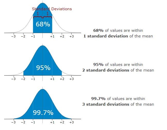
Figure 10.9: Area property of normal distribution
| mean +/- standard deviation | % of value contained |
|---|---|
| 0.745 | 50 |
| 1 | 68.26 |
| 1.96 | 95 |
| 2 | 95.44 |
| 2.58 | 99 |
| 3 | 99.73 |
In short the properties of Normal distribution
Normal distribution curve is bell shaped
Normal distribution is symmetric, not skewed.
The mean, median, and mode are all equal.
Half of the population is less than the mean and half is greater than the mean.
Area property allows you to determine the proportion of values that fall within certain distances from the mean.
Solved example
1. What is the z-score of a value of 27, given a set mean of 24, and a standard deviation of 2?
Solution
To find the z-score we need to divide the difference between the value, 27, and the mean, 24, by the standard deviation of the set, 2.
\[z = \frac{27 - 24}{2} = \frac{3}{2} = 1.5\]
This indicates that 27 is +1.5 standard deviations above the mean.