14 Small sample tests

If the sample size n is less than 30 (n < 30) it is known as small sample. For small samples the sampling distributions of statistic commonly used are χ² (Chi-square), F and t distribution. A study of sampling distribution of statistic for small samples is known as small sample theory.

Small Sample Tests (sample size (n) < 30)

14.1 Tests based on Student t distribution (t-tests)

Assumptions of t-test:

• The parent population from which the sample is drawn is normal.

• The sample is a random sample.

• The population standard deviation, σ is unknown.

14.1.1 Test for a single population mean

Consider there is a population with mean, say μ; where μ is unknown, we will take a random sample of size n from the population and calculate a sample mean, denoted as \(\overline{x}\). We want to test whether the population mean μ, which is unknown is equal to some known constant μ₀, based on the sample mean \(\overline{x}\). Here sample size is less than 30.

The null hypothesis to be tested is

H₀ : μ = μ₀

The alternative hypothesis may be either

H₁ : μ < μ₀ (called left tailed alternative)

Or

H₁ : μ > μ₀ (called right tailed alternative)

Or

H₁ : μ ≠ μ₀ (called two tailed alternative)

\[t = \frac{\overline{x} - \mu_{0}}{\frac{s}{\sqrt{n}}}\]

Where, \(s^{2} = \frac{\sum_{i = 1}^{n}\left( x_{i} - \overline{x} \right)^{2}}{n - 1}\)

Under null hypothesis t follows a t distribution with n-1 degrees of freedom

14.1.2 Decision rule for t test

Let t be the calculated value, degrees of freedom = n-1, α be the level of significance, then we reject the null hypothesis if

• |t| > t_α/2 ; for two tailed test

• t > t_α ; for right tailed test

• t < - t_α ; for left tailed test

Where t_α or t_α/2 can be obtained from the table of Student t distribution for the given degrees of freedom, n-1 and level of significance α. If the calculated value of the test statistic is less than critical values from the table. we may reject the null hypothesis. Otherwise, we may accept it.

Example 9:

Based on field experiments, a new variety of green gram is expected to give a yield of 12 quintals per hectare. The variety was tested on 10 randomly selected farmers’ fields. The yields (quintals per hectare) were recorded as 14.3, 12.6, 13.7, 10.9, 13.7, 12, 11.4, 12, 12.6, and 13.1. Do the results confirm the expectation?

Solution:

Null hypothesis, H₀ : μ = 12

Alternate hypothesis, H₁ : μ ≠ 12; two tailed test

Sample size (n) = 10

Sample mean, \(\overline{x}\) =\(\frac{\sum_{i = 1}^{n}x_{i}}{n} = (14.3+12.6+...+13.1)/10 = 126.3/10=12.63\)

Sample standard deviation (s) = 1.08536

μ₀ = 12

Level of significance, α = 0.05

Calculation of sample mean and sample standard deviation

Sl No.	Yield	\[\left( \mathbf{x}_{\mathbf{i}}\mathbf{-}\overline{\mathbf{x}}\right)\]	\[\left( \mathbf{x}_{\mathbf{i}}\mathbf{-}\overline{\mathbf{x}}\right)^{\mathbf{2}}\]
1	14.30	1.67	2.788900
2	12.60	-0.03	0.000900
3	13.70	1.07	1.144900
4	10.90	-1.73	2.992900
5	13.70	1.07	1.144900
6	12.00	-0.63	0.396900
7	11.40	-1.23	1.512900
8	12.00	-0.63	0.396900
9	12.60	-0.03	0.000900
10	13.10	0.47	0.220900
Sum = \(\sum_{i = 1}^{n}x_{i}\)	126.30	\[\sum_{i = 1}^{n}\left( x_{i} - \overline{x} \right)^{2}\]	10.601000
Mean, \(\overline{x}\) =\(\ \frac{\sum_{i = 1}^{n}x_{i}}{10}\)	12.63	\[s^{2} = \frac{\sum_{i = 1}^{n}\left( x_{i} - \overline{x} \right)^{2}}{n - 1}\]	1.177889
	NA	\[s = \sqrt{s^{2}}\]	1.085306

\[t = \frac{\overline{x} - \mu_{0}}{\frac{s}{\sqrt{n - 1}}}\]

\[t = \frac{12.63 - 12}{\frac{1.085306}{\sqrt{10 - 1}}} = \frac{0.63}{0.3432} = 1.835\]

Table value for t corresponding to 5% level of significance and 9 degrees of freedom is 2.262 (two tailed test) – see t table (Fig: 14.1) at the end of this chapter.

Since the calculated value (1.835) is less than the table value (2.262), we conclude that, we don’t have enough evidence to reject the null hypothesis. So, it can be stated that mean is 12 quintals per hectare.

Example 10: Try it by yourself

The mean weekly sales of soap bars in departmental stores were 146.3 bars per store. After an advertising campaign the mean weekly sales in 22 stores for a typical week was 153.7 and showed a standard deviation of 17.2. Was the advertisement campaign successful?

14.2 Test for equality of two means

Let there be two normally distributed populations with means µ₁ and µ₂. Let the population standard deviations be equal and unknown. Let samples of sizes n₁ and n₂ were taken from these populations. Let the sample means were 𝑥̅₁ 𝑎𝑛𝑑 𝑥̅₂ respectively. We want to test whether these population means are significantly different or not based on the sample means.

There are two cases under this situation

1. Population variances are equal

2. Population variances are unequal

Before proceeding to t-test a F test is performed to test homogeneity of population variance (See section 14.6).

14.2.1 Case when the population variances are equal (homogenous)

The null hypothesis to be tested is

H₀ : μ₁ = μ₂

The alternative hypothesis may be either

H₁ : μ₁ < μ₂ (called left tailed alternative)

Or

H₁ : μ₁> μ₂ (called right tailed alternative)

Or

H₁ : μ₁≠ μ₂ (called two tailed alternative)

We will calculate test statistic, \(t\) using the following formula.

\[t = \frac{{\overline{x}}_{1} - {\overline{x}}_{2}}{s\sqrt{\left( \frac{1}{n_{1}} + \frac{1}{n_{2}} \right)}}\]

Where, \(s^{2} = \frac{(n_{1}-1)s_{1}^2+(n_{2}-1)s_{2}^2}{n_{1} + n_{2} - 2}\); \({\overline{x}}_{1}\) and \({\overline{x}}_{2}\) are sample means from population 1 & 2, respectively.

Under null hypothesis t follows a t distribution with \(n_{1} + n_{2} - 2\) degrees of freedom. Decision rule is same as that of previous t- test (section 14.1.2).

14.2.2 Case when the population variances are unequal

The Welch t-test is an adaptation of Student’s t-test. It is used to compare the means of two groups, when the variances are different.

The null hypothesis to be tested is

H₀ : μ₁ = μ₂

The alternative hypothesis may be either

H₁ : μ₁ < μ₂ (called left tailed alternative)

Or

H₁ : μ₁> μ₂ (called right tailed alternative)

Or

H₁ : μ₁≠ μ₂ (called two tailed alternative)

We will calculate test statistic, \(t\) using the following formula.

\[t = \frac{{\overline{x}}_{1} - {\overline{x}}_{2}}{\sqrt{\left( \frac{s_{1}^{2}}{n_{1}} + \frac{s_{2}^{2}}{n_{2}} \right)}}\]

\(s_{1}\)and\({s}_{2}\) are the sample standard deviations from two populations, respectively.

The degrees of freedom of Welch t-test is calculated as follows:

\[\frac{\left( \frac{s_{1}^{2}}{n_{1}} + \frac{s_{2}^{2}}{n_{2}} \right)^{2}}{\frac{s_{1}^{4}}{n_{1}^{2}\left( n_{1} - 1 \right)} + \frac{s_{2}^{4}}{n_{2}^{2}\left( n_{2} - 1 \right)}}\]

Once the t value is determined, you have to read in the t table the critical value of Student’s t distribution corresponding to the significance level. Decision rule is same as that of previous t- test (section 14.1.2).

Example 11:

In order to compare the effectiveness of two sources of nitrogen, namely ammonium chloride and urea on grain yield of paddy, an experiment was conducted. The results on the grain yield of paddy (kg/plot) under the two treatments are given below.

Ammonium chloride: 13.4, 10.9, 11.2, 11.8, 14, 15.3, 14.2, 12.6, 17, 16.2, 16.5, 15.7

Urea: 12, 11.7, 10.7, 11.2, 14.8, 14.4, 13.9, 13.7, 16.9, 16, 15.6, 16

14.3 Paired t-test

Paired Student’s t-test is used to compare the means of two related samples. That is when you have two values (pair of values) for the same samples. For example, 20 cows received a treatment for 3 months. The question is to test whether the treatment has an impact on the milk yield of the cow at the end of the 3 months treatment. The milk yield of the 20 cows has been measured before and after the treatment. This gives us 20 sets of values before treatment and 20 sets of values after treatment. In this case, in order to test whether there is any significant difference between before and after, paired t-test can be used; as the two sets of values being compared are related. We have a pair of values for each cow (one before and the other after treatment).

Suppose we have two correlated random samples x₁, x₂, ..., x_n and y₁, y₂, ..., y_n. We want to test whether these population means are significantly different.

The Welch t-test is an adaptation of Student’s t-test. It is used to compare the means of two groups, when the variances are different.

The null hypothesis to be tested is

H₀ : μ₁ = μ₂

The alternative hypothesis may be either

H₁ : μ₁ < μ₂ (called left tailed alternative)

Or

H₁ : μ₁> μ₂ (called right tailed alternative)

Or

H₁ : μ₁≠ μ₂ (called two tailed alternative)

We will calculate test statistic, \(t\) using the following formula.

\[t = \frac{|d^̅|}{\frac{s}{\sqrt{n}}}\]

Where \(\overline{d} = \frac{\sum_{i = 1}^{n}d_{i}}{n}\); \(d_{i} = x_{i} - y_{i}\), \(s^{2} = \frac{\sum_{i = 1}^{n}\left( d_{i} - \overline{d} \right)^{2}}{n - 1}\)

Under null hypothesis t follows a t distribution with \(n - 1\) degrees of freedom. Decision rule is same as that of previous t- test (section 14.1.2).

Example 12:

In an experiment the plots were divided into two equal parts. One part received soil treatment A and the second part received soil treatment B each plot was planted with sorghum. The sorghum yield (kg/plot) was observed as shown below. Test the effectiveness of soil treatments on sorghum yield

Soil Treatment A	49	53	51	52	47	50	52	53
Soil Treatment B	52	55	52	53	50	54	54	53

Solution:

Null hypothesis, H₀ : μ₁ = μ₂, , there is no significant difference between the effects of the two soil treatments

Alternate hypothesis, H₁ : : μ₁≠ μ₂; two tailed test, there is significant difference between the effects of the two soil treatments

Level of significance, α = 0.05

\[t = \frac{|d|}{\frac{s}{\sqrt{n}}}\]

Sl No.	\[\mathbf{A}\]	\[\mathbf{B}\]	\[\mathbf{d}_{\mathbf{i}}\mathbf{= A - B}\]	\[\mathbf{d}_{\mathbf{i}}\mathbf{-}\overline{\mathbf{d}}\]	\[\left(\mathbf{d}_{\mathbf{i}}\mathbf{-}\overline{\mathbf{d}}\right)^{\mathbf{2}}\]
1	49	52	-3	-1	1
2	53	55	-2	0	0
3	51	52	-1	1	1
4	52	53	-1	1	1
5	47	50	-3	-1	1
6	50	54	-4	-2	4
7	52	54	-2	0	0
8	53	53	0	2	4
NA	NA	\[\sum_{i = 1}^{8}d_{i}\]	-16	\[\sum_{i = 1}^{8}\left( d_{i} - \overline{d} \right)^{2}\]	12
NA	NA	\[\overline{d} = \frac{\sum_{i = 1}^{8}d_{i}}{n} = \frac{- 16}{8}\]	\(\overline{d} =\)-2	\[s^{2} = \frac{\sum_{i = 1}^{8}\left( d_{i} - \overline{d} \right)^{2}}{n - 1}\]	\(s^{2}\)=1.7143
NA	NA				\(s = \sqrt{1.7143}\) =1.309

\[t = \frac{| - 2|}{\frac{1.309}{\sqrt{8}}}\]

\[= \frac{2}{\frac{1.309}{2.828}}\]

\[= \frac{2}{0.4629}\]

\[= 4.321\]

Table value of t for 7 degrees of freedom at 5% level of significance is 2.365

As calculated value (4.321) is greater than table value (2.365). We reject the null hypothesis H₀. We conclude that the is significant difference between the two soil treatments between A and B. Soil treatment B increases the yield of sorghum significantly.

Example 13: Try it by yourself

A certain stimulus administered to each of 12 patients resulted in the following increase of Blood pressure: 5, 2, 8, -1, 3, 0, -2, 1, 5, 0, 4, 6. Can it be concluded that the stimulus will, in general be accompanied by an increase in blood pressure? (tip: difference \(d_{i}\) is given)

14.4 Testing the significance of correlation coefficient

Let there be two normally distributed populations with means µ₁ and µ₂ and standard deviations be σ₁ and σ₂ respectively. Let the correlation between two populations be ρ. We want to test the null hypothesis that population correlation coefficient is zero (ρ =0). We can use t- test for the purpose. If we don’t have enough evidence from our sample to reject the null hypothesis, we may conclude that there is a significant correlation between populations (ρ ≠ 0).

The null hypothesis to be tested is

H₀ : ρ = 0

The alternative hypothesis

H₁ : ρ ≠ 0 (two tailed alternative)

\[t = \frac{r\sqrt{n - 2}}{\sqrt{1 - r^{2}}}\]

Under null hypothesis t follows a t distribution with \(n - 2\) degrees of freedom. We reject the null hypothesis, if the calculated value is greater than table value of t corresponding to \(n - 2\) degrees of freedom and level of significance (α). our case α = 0.05

Example 14:

A coefficient of correlation of 0.2 is derived from a random sample of 625 pairs of observations. Test whether the population correlation coefficient is significant or not.

Solution:

Null hypothesis, H₀ : ρ = 0 (Population correlation coefficient is zero)

Alternative hypothesis, H₁ : ρ ≠ 0 (Population correlation coefficient is not zero)

Sample correlation coefficient (\(r\)) = 0.2

Number of pairs (n) = 625

\[t = \frac{r\sqrt{n - 2}}{\sqrt{1 - r^{2}}}\]

\[= \frac{0.2\sqrt{625 - 2}}{\sqrt{1 - 0.04}}\ = 5.095\]

Sample size is so large (>30) t distribution can be approximated to a z distribution. Critical value for two tailed test at 5% level of significance is 1.96. So the calculated value is more than 1.96, we reject the null hypothesis and conclude that, there is a significant correlation in population.

14.5 Chi square test (χ²)

Chi-square tests are based on the sampling distribution called chi-square distribution (χ² distribution). χ²tests are based on the following assumptions

1. The sample observations are independent.

2. The total frequency should be reasonably large, say, greater than 50.

3. The theoretical cell frequencies should not be less than 5. If any theoretical cell frequency is less than 5, then for the application χ²tests, it is pooled with the preceding or succeeding frequencies so that the pooled frequency is more than 5 and finally adjust the degrees of freedom lost in pooling.

4. Constraints on the cell frequencies should be linear. (eg., ∑ 𝑂_𝑖 = ∑ 𝐸_𝑖 (where O_i and E_i represents the observed and expected frequencies)

Note:

The χ² tests do not make any assumptions regarding the parent population from which the observations are taken. Such tests do not involve any population parameter. Hence these tests are known as non-parametric tests or distribution free tests.

Degrees of freedom in χ² tests: Degrees of freedom in χ² tests refers to the number of independent variates which make up the statistic. The degrees of freedom in general is the total number of observations less the number of independent constraints imposed on the observations. For example, if k is the number of independent constraints in a set of data on n observations, then degrees of freedom = n-k.

Three important chi-square tests:

• Chi-square test for goodness of fit.

• Chi-square test for independence of attributes.

• Chi-square test for a variance.

14.5.1 Chi square test (χ²) for goodness of fit

A very powerful test for testing the significance of the discrepancy between theory and experiment was given by Prof. Karl Pearson in 1900 and is known as “χ² tests for goodness of fit”.

We want to test the null hypothesis, H₀: There is no significance between the theory and experiment

Against the alternative hypothesis H₁: There is significance between the theory and experiment

If O_i (i=1,2,...,n) is a set of observed frequencies and E_i (i=1,2,...,n) is the corresponding set of expected (theoretical) frequencies, then Karl Pearson’s chi-square test statistic is given by

\[\chi^{2} = \sum_{i = 1}^{n}\frac{\left( O_{i} - E_{i} \right)^{2}}{E_{i}}\]

Here O_i represents the i^th observed frequency and E_i represents the corresponding expected frequency according to the assumption regarding the theory behind the data. Under null hypothesis chi-square follows chi-square distribution with n-1 degrees of freedom.

14.5.1.1 Decision rule for goodness of fit test

Let \(\chi_{\text{cal}}^{2}\) be the calculated value, degrees of freedom = n-1, α be the level of significance, then we reject the null hypothesis if \(\chi_{\text{cal}}^{2}\) > \(\chi_{\text{tab}}^{2}\); where \(\chi_{\text{tab}}^{2}\) is the table value of \(\chi^{2}\)at n-1 degrees of freedom. In case of \(\chi^{2}\) test only one tailed test is used.

Example 15:

In plant genetics, our interest may be to test whether the observed segregation ratios deviate significantly from the mendelian ratios. In such situations we want to test the agreement between the observed and theoretical frequency, such test is called as test of goodness of fit. In a cross between parents of the genetic constitution AAbb and aaBB, the phenotypes in the sample is classified as follows:

AB	Ab	aB	ab	Total
87	29	32	12	160

They are expected to occur in a 9: 3: 3: 1 ratio. Do the data agree with the theoretical ratio?

Solution:

Phenotypes	AB	Ab	aB	ab	Total
Observed (Oi)	87	29	32	12	160.000
Expected (Ei)	\(\frac{9}{16}\ \times 160\) =90	\(\frac{3}{16}\ \times 160\) =30	\(\frac{3}{16}\ \times 160\) =30	\(\frac{1}{16}\ \times 160\) =10	160.000
\[\mathbf{O}_{\mathbf{i}}\mathbf{-}\mathbf{E}_{\mathbf{i}}\]	-3	-1	2	2	NA
\[\left( \mathbf{O}_{\mathbf{i}}\mathbf{-}\mathbf{E}_{\mathbf{i}} \right)^{\mathbf{2}}\]	9	1	4	4	NA
\[\frac{\left( \mathbf{O}_{\mathbf{i}}\mathbf{-}\mathbf{E}_{\mathbf{i}} \right)^{\mathbf{2}}}{\mathbf{E}_{\mathbf{i}}}\]	0.11	0.033	0.133	0.4	0.676

\[\chi^{2} = \sum_{i = 1}^{n}\frac{\left( O_{i} - E_{i} \right)^{2}}{E_{i}}\]

\[\chi^{2} = 0.676\]

\(\chi_{\text{cal}}^{2}\)= 0.676, table value of chi-square for 4-1=3 degrees of freedom and 5% level of significance is 7.815. We won’t reject the null hypothesis, H₀: There is no significance between the theory and experiment. Conclude that data follows 9:3:3:1 ratio.

Example 16: Try by yourself

The number of yeast cells counted in a haemocytometer is compared to the theoretical value is given below. Does the experimental result support the theory.

Yeast per cell	Observed Frequency	Expected Frequency
0	103	106
1	143	141
2	98	93
3	42	41
4	8	14
5	6	5

14.5.2 Chi square test (χ²) for independence of attributes

The Chi-square test of independence checks whether two attributes are likely to be related or not. For example, chemical treatment and germination can be two attributes. If we want to know whether chemical treatment has any influence on germination, we can use chi-square test. For this purpose, we need the data arranged in the form of a contingency table.

14.5.2.1 Contingency table

A contingency table consists of a collection of cells containing counts. A contingency table is a tabular representation of categorical data. A contingency table usually shows frequencies for particular combinations of values of two discrete random variables X and Y. Each cell in the table represents a mutually exclusive combination of X-Y values.

Example 17: Contingency table

In order to determine the possible effect of a chemical treatment on the rate of germination of cotton seeds a pot culture experiment was conducted. The results are given below in the form of a contingency table is given below. (X = Germination, Y = Chemical Treatment). Attribute X has two class X₁ = Germinated, X₂ = Not germinated. Attribute Y has two class Y₁ = Treated, Y₂ = Untreated.

	X=Germination
Y= Chemical treatment	X/Y	Germinated(X1)	Not Germinated(X2)	Total
	Treated(Y1)	118	22	140
	Untreated(Y2)	120	40	160
	Total	238	62	300

Let us consider two attributes A & B, A divided into r classes A₁, A₂, ..., A_r and B divided into s classes B₁, B₂, ..., B_s. The various cell frequencies can be expressed in the form of a table (called r × s contingency table) as shown below.

A.B	A1	A2	…..	Ar	Total
B1	(A1 B1)	(A2 B1)	. . .	(Ar B1)	(B1)
B2	(A1 B2)	(A2 B2)	. . .	(Ar B2)	(B2)
.	.	.	.	.	.
.	.	.	.	.	.
.	.	.	.	.	.
Bs	(A1 Bs)	(A2 Bs)	. . .	(Ar Bs)	(Bs)
Total	(A1)	(A2)	. . .	(Ar)

(A_iB_j) = The number of persons (items) possessing attributes A_i (i =1,2,..., r) and B_j (j =1,2,...,s)

(A_i) = The number of persons (items) possessing attribute A_i ( i =1,2,..., r)

(B_j) = The number of persons (items) possessing attribute B_j (j =1,2,..., s)

∑(A)_𝑖 = ∑(B)_𝑗 = 𝑁, is the total frequency.

14.5.2.2 Expected frequencies

The expected frequencies corresponding to each observed frequency (A_iB_j) are calculated from the formula,

\[E_{\text{ij}} = \frac{\left( A_{i} \right)\left( B_{j} \right)}{N}\]

14.5.2.3 Degrees of freedom

Degrees of freedom for an r × s contingency table = (r – 1)(s – 1)

Test procedure

The null hypothesis to be tested is H₀: The two attributes under consideration are independent.

The alternative hypothesis is H₁: The two attributes under consideration are not independent.

Test statistic used is

\[\chi^{2} = \sum_{i = 1}^{r}{\sum_{j = 1}^{s}\frac{\left( O_{\text{ij}} - E_{\text{ij}} \right)^{2}}{E_{\text{ij}}}}\]

Where,

\(O_{\text{ij}}\) = observed frequencies

\(E\_{\text{ij}}\)= Expected frequencies

s = number of rows

r = number of columns

It can be verified that \(\sum_{i = 1}^{r}{\sum_{j = 1}^{s}O_{\text{ij}}} = \sum_{i = 1}^{r}{\sum_{j = 1}^{s}E_{\text{ij}}}\)

Under null hypothesis test statistic follows a chi-square distribution with (r – 1)×(s – 1) degrees of freedom. Decision rule is same as Chi square for goodness of fit.

Example 18:

In a survey, a random sample of 198 farms were classified in to three classes according to tenure status as: owned, rented and mixed. They were also classified according to the level of soil fertility as: high fertile, moderately fertile and low fertile farms. The results are given below. Test whether tenure status depends on soil fertility

	Tenure Status
Soil fertility	Owned	Rented	Mixed	Total
High	40	12	10	62
Moderate	22	10	14	46
Low	22	26	42	90
Total	84	48	66	198

Solution:

Calculation of expected values (\(E_{\text{ij}})\) for each cell by multiplying corresponding row total and column total divided by total frequency in the above table

X	Owned	Rented	Mixed
High	\(\frac{62\ \times 84}{198} =26.3\)	\(\frac{62\ \times 48}{198} =15.0\)	\(\frac{62\ \times 66}{198} =20.7\)
Moderate	\(\frac{46\ \times 84}{198} =19.5\)	\(\frac{46\ \times 48}{198} =11.2\)	\(\frac{46\ \times 66}{198} =15.3\)
Low	\(\frac{90\ \times 84}{198} =38.2\)	\(\frac{90\ \times 48}{198} =21.8\)	\(\frac{90\ \times 66}{198} =30.0\)

\[O_{\text{ij}}\]	\[E_{\text{ij}}\]	\[O_{\text{ij}} - E_{\text{ij}}\]	\[\left(O_{\text{ij}} - E_{\text{ij}} \right)^{2}\]	\[\frac{\left( O_{\text{ij}} - E_{\text{ij}} \right)^{2}}{E_{\text{ij}}}\]
40	26.3	13.7	187.6	7.1
12	15.0	-3.0	9.2	0.6
10	20.7	-10.7	113.8	5.5
22	19.5	2.5	6.2	0.3
10	11.2	-1.2	1.3	0.1
14	15.3	-1.3	1.8	0.1
22	38.2	-16.2	261.9	6.9
26	21.8	4.2	17.5	0.8
42	30.0	12.0	144	4.8
NA	NA	NA	\[\chi_{\text{cal}}^{2} =\]	26.3

\(\chi_{\text{cal}}^{2}\)= 26.3, table value of chi-square for (3-1)(3-1) = 4 degrees of freedom and 5% level of significance is 9.488. Since the calculated value is greater than table value, we reject the null hypothesis, and conclude that the two attributes under consideration are not independent.

14.5.3 Chi-square test for 2×2 contingency table

2 x 2 contingency table

When the number of rows and number of columns are equal to 2; it is termed as 2 x 2 contingency table. It will be in the following form as shown in example 17. General form can be represented as shown below. Consider two attributes A and B with classes A₁, A₂ and B₁, B₂ respectively. a, b, c, d are the frequencies in each cell

	A1	A2	Row Total
B1	a	b	R1= a+b
B2	c	d	R2 = c+d
Column Total	C1= a+c	C2 = b+d	n = a+b+c+d

R₁, R₂ and C₁, C₂ are row totals and column totals respectively. n is the total number of observations.

In case of 2 x 2 contingency table \(\chi^{2}\) can be directly found using the short cut formula.

The null hypothesis to be tested is H₀: The two attributes under consideration are independent.

The alternative hypothesis is H₁: The two attributes under consideration are not independent.

\[\chi^{2} = \frac{n\left( ad - bc \right)^{2}}{C_{1}C_{2}R_{1}R_{2}}\]

Under null hypothesis test statistic follows a chi-square distribution with (2 – 1) × (2 – 1) = 1 degrees of freedom.

14.5.3.1 Yate’s correction for continuity

In a 2 X 2 contingency table, the number of degrees of freedom is (2-1) × (2-1) = 1. If any one of the cell frequencies is less than 5, then, use of pooling method results in \(\chi^{2}\) with 0 degrees of freedom (1 degrees of freedom is lost due to pooling) which is meaningless. In this case we apply a correction due to Yates which is usually known as Yates’ correction for continuity. The Yate’s correction is made by adding 0.5 to the least cell frequency and adjusting the other cell frequencies so that the column and row totals remain same. The formula for the test statistic in equation (15) is now modified and is given as below.

Test statistic used is

\[\chi^{2} = \frac{{n\left( \left| ad - bc \right| - \frac{n}{2} \right)}^{2}}{C_{1}C_{2}R_{1}R_{2}}\]

Solution to Example 17

H₀: The treatment does not improve the germination rate of cotton seeds. (independent)

H₁: The chemical treatment improves the germination rate of cotton seeds.

\[\chi^{2} = \frac{{300\left( \left| 118 \times 40 - 22 \times 120 \right| - \frac{300}{2} \right)}^{2}}{238 \times 62 \times 140 \times 160}\]

\[= 3.927\]

\(\chi_{\text{cal}}^{2}\)= 3.927, table value of chi-square for (2-1) × (2-1) = 1 degrees of freedom and 5% level of significance is 3.841. Since the calculated value is less than table value, we don’t have enough evidence to reject the null hypothesis. The chemical treatment will not improve the germination rate of cotton seeds significantly.

Example 19: Try it for yourself

In an experiment on the effect of a growth regulator on fruit setting in muskmelon, the following results were obtained. Test whether the fruit setting in muskmelon and the application of growth regulator are independent at 5% level.

	Fruit set	Fruit not set
Treated	16	9
Control	4	21

14.5.4 Chi-square test for a population variance

Consider there is a normal population with mean, say μ and variance σ², where μ and σ² are unknown, we will take a random sample of size n from the population. We want to test whether the population variance σ², which is unknown is equal to some known constant σ²₀, based on the sample variance.

Null hypothesis H₀: σ² = σ²₀

Against the alternative hypothesis H₁: σ² > σ²₀

The test statistic is

\[\chi^{2} = \frac{ns^{2}}{\sigma_{0}^{2}}\]

Where \(s^{2} = \frac{\sum_{i = 1}^{n}\left( x_{i} - \overline{x} \right)^{2}}{n - 1}\)is the sample variance

Under null hypothesis test statistic follows a chi-square distribution with n-1 degrees of freedom. Decision rule is same as in section 3.1.1

Example 20: Try it for yourself

Test the null hypothesis that σ² = 0.16 against the alternative hypothesis σ² > 0.16, given that \(s^{2}\) = 0.01719 for a random sample of size 11 from a normal population.

14.6 F - test for testing equality of two population variances

Let there be two normally distributed populations with means µ₁ and µ₂ and variances be σ₁² and σ₂² respectively. Let samples of sizes n₁ and n₂ were taken from these populations. We want to test whether these population variances are significantly different or not based on the sample variances.

Null hypothesis H₀: σ²₁ = σ²₂

Against the alternative hypothesis H₁: σ²₁ > σ²₂

Test statistic is

\[F = \frac{s_{1}^{2}}{s_{2}^{2}}\]

Under null hypothesis test statistic follows a F distribution with \(n_{1} - 1\) and \(n_{2} - 1\) degrees of freedom.

14.6.1 Decision rule for F - test

If the calculated value is greater than table value of F at specified level of significance and two degrees of freedom (i.e. \(n_{1} - 1\) and \(n_{2} - 1\)) we reject the null hypothesis.

Note:

If \(s_{2}^{2} >\) \(s_{1}^{2}\) the test statistic will be

\[F = \frac{s_{2}^{2}}{s_{1}^{2}}\]

Under null hypothesis test statistic follows a F distribution with \(n_{2} - 1\) and \(n_{1} - 1\) degrees of freedom.

Example 20: Try it for yourself

For a random sample representing one normal population, we have \(n_{1}\) = 11, and \(s_{1}^{2}\) = 21.87. For another random sample representing the second normal population, we have\(\ n_{2}\)= 8 and \(s_{2}^{2}\) = 15.36. Test the equality of variances.

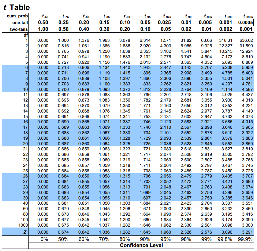
Figure 14.1: t table

 
 
 

“Like dreams, statistics are a form of wish fulfillment”:-Jean Baudrillard