6 Skewness and Kurtosis
In the previous chapter we have learned numerical measures of central tendency and dispersion, but what about measures of shape?
The histogram can give you a general idea on the shape of the distribution of values in your data. But we need some numerical measures to identify the shape of the distribution. The numerical measures which deal with the shape of the distribution are Skewness and Kurtosis.
6.1 Skewness
Skewness is a measure of symmetry, or more precisely, the lack of symmetry. Then you may ask, what will a symmetric distribution looks like. Histogram of a symmetric distribution is showed below:
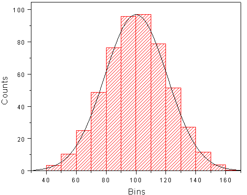
Figure 6.1: Histogram of a symmetric distribution
A distribution, or data set, is symmetric if it looks the same to the left and right of the centre point. In our discussion we are including only unimodal cases.
For a symmetric distribution skewness = 0; mean = median = mode
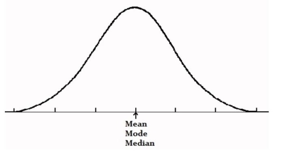
Figure 6.2: symmetric distribution
Example of a data set with skewness = 0 (symmetric distribution)
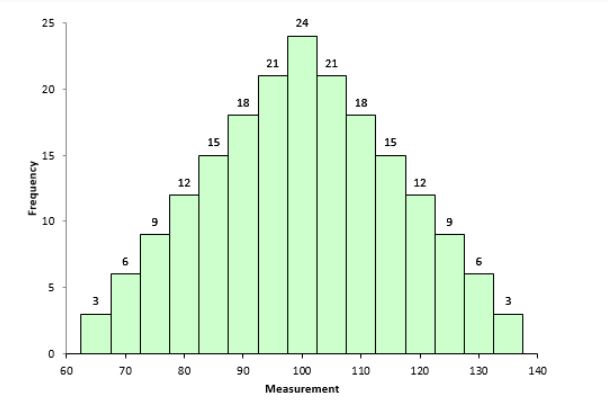
Figure 6.3: Data set with skewness = 0
6.1.1 Left-skewed or negatively skewed
For negatively skewed data set or distribution, the left tail is longer; the mass of the distribution is concentrated on the right of the figure. The distribution is said to be left-skewed, left-tailed, or skewed to the left, considering that there is a long tail in the left side. See the figure below, you can also see Mean < Median < Mode.
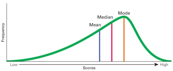
Figure 6.4: Left skewed or negatively skewed distribution
Example of a data set with negative skewness
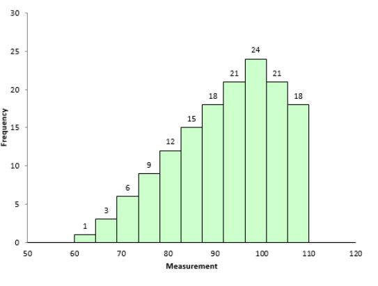
Figure 6.5: Negatively skewed data set
6.1.2 Right-skewed or positively skewed
For positively skewed data set or distribution, the right tail is longer; the mass of the distribution is concentrated on the left of the figure. The distribution is said to be right-skewed, right-tailed, or skewed to the right, considering that there is a long tail in the right side. See the figure below, you can also see Mean > Median > Mode
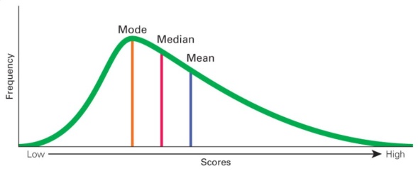
Figure 6.6: Right skewed or positively skewed distribution
Example of a data set with positive skewness
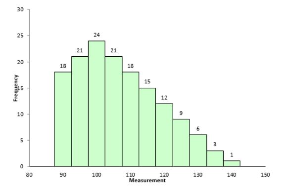
Figure 6.7: Data set with positive skewness (right skewed)
6.2 Measures of Skewness
The direction and extent of skewness can be measured in various ways. We shall discuss four measures.
6.2.1 Karl Pearson’s coefficient of Skewness (\(S_{k}\))
You have noticed that the mean, median and mode are not equal in a skewed distribution. The Karl Pearson’s measure of skewness is based upon the divergence of mean from mode in a skewed distribution.
\[S_{k} = \frac{mean - mode}{\text{standard deviation}}\]
The sign of \(S_{k}\) gives the direction of skewness and its magnitude gives the extent of skewness. If \(S_{k}\) > 0, the distribution is positively skewed, and if \(S_{k}\) < 0 it is negatively skewed.
In the above formula since mode is used, there is a problem that if mode is not defined for a distribution we cannot find \(S_{k}\). But empirical relation between mean, median and mode states that, for a moderately symmetrical distribution \(\ mean - mode \approx 3(mean - median)\). So the above formula can be written as
\[S_{k} = \frac{3(mean - median)}{\text{standard deviation}}\]
Example 6.1: Compute the Karl Pearson’s coefficient of skewness from the following data:
| Height (x) | frequency (f) |
|---|---|
| 58 | 10 |
| 59 | 18 |
| 60 | 30 |
| 61 | 42 |
| 62 | 35 |
| 63 | 28 |
| 64 | 16 |
| 65 | 8 |
| Height (\(x_{i}\)) | frequency (\(f_{i}\)) | \[f_{i}x_{i}\] | \[f_{i}x_{i}^{2}\] |
|---|---|---|---|
| 58 | 10 | 580 | 33640 |
| 59 | 18 | 1062 | 62658 |
| 60 | 30 | 1800 | 108000 |
| 61 | 42 | 2562 | 156282 |
| 62 | 35 | 2170 | 134540 |
| 63 | 28 | 1764 | 111132 |
| 64 | 16 | 1024 | 65536 |
| 65 | 8 | 520 | 33800 |
| Sum | 187 | 11482 | 705588 |
Mean, \(\overline{x} = \frac{\sum_{i = 1}^{n}{f_{i}x_{i}}}{\sum_{i = 1}^{n}f_{i}}\) = \(\frac{11482}{187} = 61.40\)
\({sample\ variance,\ s}^{2} = \frac{1}{n - 1}\left\{ \sum_{i = 1}^{n}{{f_{i}x}_{i}^{2} - \frac{1}{n}}\left( \sum_{i = 1}^{n}{f_{i}x}_{i} \right)^{2} \right\}\)= \(\frac{705588 - \frac{\left( 11482 \right)^{2}}{187}}{186} = 3.0976\)
\(standard\ deviation,\ s = \sqrt{3.0976} = 1.76\)
Median: See in the cumulative frequencies, the value just greater than\(\ \left( \frac{n + 1}{2} \right)\) , then the corresponding value of \(x\) is \(Q_{2}\), median
\(\left( \frac{n + 1}{2} \right) = \frac{187 + 1}{2}= \frac{188}{2}\) = 94
| Height (x) | frequency (f) | cumulative frequency |
|---|---|---|
| 58 | 10 | 10 |
| 59 | 18 | 28 |
| 60 | 30 | 58 |
| 61 | 42 | 100 |
| 62 | 35 | 135 |
| 63 | 28 | 163 |
| 64 | 16 | 179 |
| 65 | 8 | 187 |
\[S_{k} = \frac{3(mean - median)}{\text{standard deviation}}\]
\[S_{k} = \frac{3(61.40 - 61)}{1.179} = \frac{1.2}{1.179} = 0.68\]
Hence, the Karl Pearson’s coefficient of skewness \(S_{k}\)=\(1.017\), Thus the distribution is positively skewed.
6.2.2 Bowley’s measure of Skewness (SQ)
Karl Pearson’s coefficient of skewness is most commonly used skewness measure. However, in order to use it you must know the mean, mode (or median) and standard deviation for your data. Sometimes you might not have that information; instead you might have information about quartiles. If that’s the case, you can use Bowley’s measure of Skewness as an alternative to find out more about the asymmetry of your distribution. It’s very useful if you have extreme data values (outliers) or if you have an open-ended distribution.
\[{Bowley’s\ measure\ of\ Skewness,\ S}_{Q} = \frac{\left( Q_{3} - Q_{2} \right) - \left( Q_{2} - Q_{1} \right)}{\left( Q_{3} - Q_{2} \right) + \left( Q_{2} - Q_{1} \right)}\]
Where \(Q_{1}\)= 1st quartile; \(Q_{2}\) = median; \(Q_{3}\)= 3rd quartile
Equation can be further modified into
\[S_{Q} = \frac{Q_{3} - 2Q_{2} + Q_{1}}{Q_{3} - Q_{1}}\]
\(S_{Q}\)= 0 means that the curve is symmetrical.
\(S_{Q}\) > 0 means the curve is positively skewed.
\(S_{Q}\)< 0 means the curve is negatively skewed.
For Example 6.1 given above, Bowley’s measure of Skewness can be calculated as follows
| Height (x) | frequency (f) | cumulative frequency |
|---|---|---|
| 58 | 10 | 10 |
| 59 | 18 | 28 |
| 60 | 30 | 58 |
| 61 | 42 | 100 |
| 62 | 35 | 135 |
| 63 | 28 | 163 |
| 64 | 16 | 179 |
| 65 | 8 | 187 |
Calculation of\(\text{Q}_{1}\), \(Q_{2}\), \(Q_{3}\) is given in Section 4.5.1
\[{Q}_{1} = 60\]
\[Q_{2} = 61\]
\[Q_{3} = 63\]
\[S_{Q} = \frac{63 - (2 \times 61) + 60}{63 - 60} = \ \frac{1}{3} = 0.33\]
Since \(S_{Q}\) > 0 means the curve is positively skewed.
6.2.3 Kelly’s Measure of Skewness (Sp)
Bowley’s measure of skewness is based on the middle 50% of the observations; it leaves 25% of the observations on each extreme of the distribution. As an improvement over Bowley’s measure, Kelly has suggested a measure based on Percentiles, including P10 and P90 so that only 10% of the observations on each extreme are ignored.
\[{Kelly's\ Measure\ of\ Skewness,\ S}_{p} = \frac{\left( P_{90} - P_{50} \right) - \left( P_{50} - P_{10} \right)}{\left( P_{90} - P_{50} \right) + \left( P_{50} - P_{10} \right)}\]
6.2.4 Measure based on moments
Before going into measuring skewness using moments, one should know what a moment is:
6.2.4.1 Moments
The rthmoment about mean of a distribution, denoted by μr is given by
\[\mu_{r} = \frac{\sum_{i = 1}^{N}{f_{i}\left( x_{i} - \overline{x} \right)^{r}}}{N}\]
Where \(f_{i}\) is the frequency of ith observation or class mark\(\ x_{i}\), \(N = \sum_{}^{}f_{i}\), number of observations
Moment about mean is also called as Central Moment
If r = 0, \(\mu_{0} = \frac{\sum_{i = 1}^{N}{f_{i}\left( x_{i} - \overline{x} \right)^{0}}}{N}\) = 1
If r = 1, \(\mu_{1} = \frac{\sum_{i = 1}^{N}{f_{i}\left( x_{i} - \overline{x} \right)^{1}}}{N}\) = 0 (sum of deviation about mean is zero)
If r = 2, \(\mu_{2} = \frac{\sum_{i = 1}^{N}{f_{i}\left( x_{i} - \overline{x} \right)^{2}}}{N}\) = \(\sigma^{2}\), Population variance
In short values of following moments about mean are
|
Moments about mean (central moment) |
Value |
|---|---|
| \[\mu_{0}\] | 1 |
| \[\mu_{1}\] | 0 |
| \[\mu_{2}\] | \(\sigma^{2}\) |
For the Example 6.1 given above, calculate third central moment, \(\mu_{3}\)
| Height (\(x_{i}\)) | frequency (\(f_{i}\)) | \[\left( x_{i}-\overline{x} \right)^{3}\] | \[{f_{i}\left( x_{i}-\overline{x}\right)}^{3}\] |
|---|---|---|---|
| 58 | 10 | -39.304 | -393.040 |
| 59 | 18 | -13.824 | -248.832 |
| 60 | 30 | -2.744 | -82.320 |
| 61 | 42 | -0.064 | -2.688 |
| 62 | 35 | 0.216 | 7.560 |
| 63 | 28 | 4.096 | 114.688 |
| 64 | 16 | 17.576 | 281.216 |
| 65 | 8 | 46.656 | 373.248 |
| Sum | 187 | 12.608 | 49.832 |
Mean = 61.40
\[\mu_{3} = \frac{\sum_{i = 1}^{N}{f_{i}\left( x_{i} - \overline{x} \right)^{3}}}{N} = \ \frac{49.832}{187} = 0.266\]
6.2.4.2 Moment measure of skewness \(\mathbf{(}\beta_{1}\text{and}\)\(\gamma_{1}\mathbf{)}\)
The moment measure of skewness is based on the property that, for a symmetrical distribution, all odd ordered central moments are equal to zero. We note that \(\mu_{1}\) = 0, for every distribution, therefore, the lowest order moment that can provide an absolute measure of skewness is \(\text{μ}_{3}\). So measures of skewness are based on \(\text{μ}_{3}\).
\[\beta_{1} = \frac{\mu_{3}^{2}}{\mu_{2}^{3}}\]
Pronounced as ‘beta one’
\(\beta_{1}\)= 0 means that the curve is symmetrical. The greater the value of \(\beta_{1}\)the more skewed the distribution. One serious limitation of \(\beta_{1}\)is that it cannot tell the direction of skewness, i.e., whether it is positive or negative. Since \(\text{μ}_{2}\) is always positive and \(\mu_{3}^{2}\) is positive, \(\beta_{1}\) will be positive always. This drawback is removed by calculating\(\text{γ}_{1}\), called as Karl Pearson’s\(\text{ γ}_{1}\), pronounced as ‘gamma one’.
\[\gamma_{1} = \sqrt{\beta_{1}} = \frac{\mu_{3}}{\mu_{2}^{3}}\]
If \(\mu_{3}\) is positive \(\gamma_{1}\) is positive, If \(\mu_{3}\) is negative \(\gamma_{1}\) is negative
\(\gamma_{1}\)= 0 means that the curve is symmetrical.
\(\gamma_{1}\) > 0 means the curve is positively skewed.
\(\gamma_{1}\)< 0 means the curve is negatively skewed.
For the Example 6.1 given above, skewness can be examined as below
\(\mu_{3}\)= 0.226
\(\mu_{2}\)= 3.123
\(\beta_{1} = \frac{\mu_{3}^{2}}{\mu_{2}^{3}}\) = \(\frac{\left( 0.226 \right)^{2}}{\left( 3.123 \right)^{3}} = \ \frac{0.051}{30.46} = 0.0016\)
\(\gamma_{1} = \sqrt{\beta_{1}} = \ \sqrt{0.0016} = + 0.04\)
Since \(\mu_{3}\) is positive \(\gamma_{1}\)is positive. Since \(\gamma_{1}\)is slightly greater than 0, distribution is a slightly skewed to right.
6.3 Kurtosis
Kurtosis is another measure of the shape of a distribution. Whereas skewness measures the lack of symmetry of the frequency curve of a distribution, kurtosis is a measure of the relative peakedness of its frequency curve. Various frequency curves can be divided into three categories depending upon the shape of their peak.
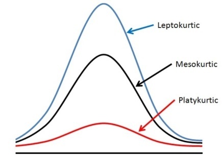
Figure 6.8: Three categories of frequency curves depending upon the shape of their peak
Kurtosis refers to degree of flatness or peakedness of the curve. It is measured relative to the peakedness of normal curve. The normal curve is considered as mesokurtic. If a curve is more peaked than normal curve, it is called leptokurtic. If a curve is more flat-topped than normal curve, it is called platykurtic.
The condition of peakedness (leptokurtic) or flatness (platykurtic) is called kurtosis of excess.
Measure of kurtosis is given by ‘beta two’ given by Karl Pearson
\(\beta_{2} = \frac{\mu_{4}}{\mu_{2}^{2}}\)
Where \(\mu_{4}\) is the 4th central moment, \(\mu_{2}\) is the 2nd central moment
\(\beta_{2}\)= 3 means that the curve is mesokurtic.
\(\beta_{2}\) > 3 means the curve is leptokurtic.
\(\beta_{2}\)< 3 means the curve is platykurtic.
Another measure of kurtosis is gamma two, \(\gamma_{2} = \beta_{2} - 3\)
\(\gamma_{2}\)= 0 means that the curve is mesokurtic.
\(\gamma_{2}\) > 0 means the curve is leptokurtic.
\(\gamma_{2}\)< 0 means the curve is platykurtic.
For the Example 6.1 given above, kurtosis can be examined as follows
| Height (\(x_{i}\)) | frequency (\(f_{i}\)) | \[\left( x_{i}-\overline{x} \right)^{4}\] | \[{f_{i}\left( x_{i}-\overline{x}\right)}^{4}\] |
|---|---|---|---|
| 58 | 10 | 133.6336 | 1336.3360 |
| 59 | 18 | 33.1776 | 597.1968 |
| 60 | 30 | 3.8416 | 115.2480 |
| 61 | 42 | 0.0256 | 1.0752 |
| 62 | 35 | 0.1296 | 4.5360 |
| 63 | 28 | 6.5536 | 183.5008 |
| 64 | 16 | 45.6976 | 731.1616 |
| 65 | 8 | 167.9616 | 1343.6930 |
| Sum | 187 | 391.0208 | 4312.7470 |
Mean, \(\overline{x}\)= 61.40
\(\mu_{2}\) = 3.123 (calculation shown in previous example)
\(\mu_{4} = \frac{\sum_{i = 1}^{N}{f_{i}\left( x_{i} - \overline{x} \right)^{4}}}{N} = \frac{4312.747}{187} = 23.062\)
\(\beta_{2} = \frac{\mu_{4}}{\mu_{2}^{2}} = \frac{23.062}{\left( 3.123 \right)^{2}} = 2.364\)
\(\beta_{2}\) is 2.364, which is close to 3, distribution can be considered slightly platykurtic close to symmetric.
You can verify the frequency curve of Example 6.1 below, it can be seen that it is slightly right tailed (positively skewed)
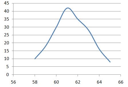
Figure 6.9: frequency curve of Example 6.1